Houze Robert A., Jr. Cloud Dynamics

Подождите немного. Документ загружается.

11.2 Circulation at a Front 459

x--

cold warm

~"'''"'"'~"'~"'"'~",,~"'"'"'"'"'"'"'~"'"'"'"'"'"'"'"'~

x, X

X--

(a)

(b)

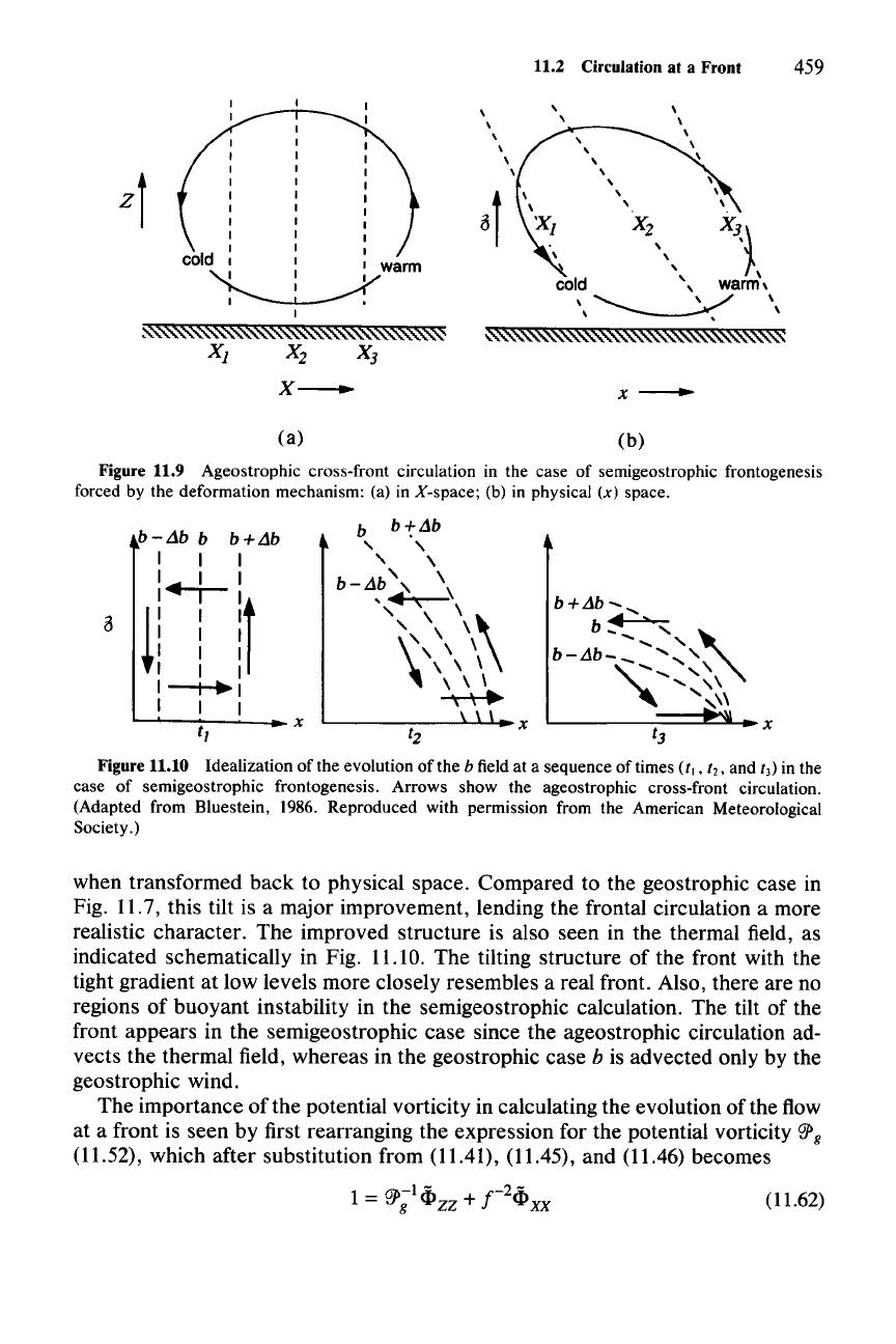
Figure 11.9 Ageostrophic cross-front circulation in the case of semigeostrophic frontogenesis

forced by the deformation mechanism: (a) in

X-space; (b) in physical

(x)

space.

b-Lib

b+Lib

I I I

I..J-I

I I I

I I

I I I

b b + Lib

, ,

b-Lib

'~\

,,'

\ \

\'<\

,\ \ \

b+Lib

.....

b~,~

b-Lib-

" "

...........

, ,

',\\

L----==~i....x

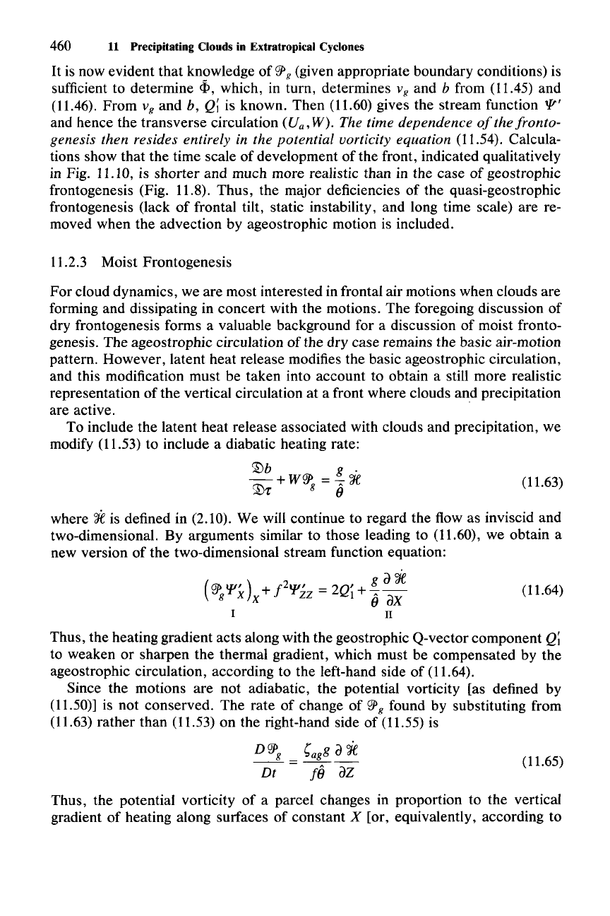
Figure 11.10 Idealization of the evolution of the b field at a sequence oftimes

(tl

, t2, and t) in the

case of semigeostrophic frontogenesis. Arrows show the ageostrophic cross-front circulation.

(Adapted from Bluestein,

1986. Reproduced with permission from the American Meteorological

Society.)

when transformed back to physical space. Compared to the geostrophic case in

Fig. 11.7, this tilt is a major improvement, lending the frontal circulation a more

realistic character. The improved structure is also seen in the thermal field, as

indicated schematically in Fig. 11.10. The tilting structure of the front with the

tight gradient at low levels more closely resembles a real front. Also, there are no

regions of buoyant instability in the semigeostrophic calculation. The tilt of the

front appears in the semigeostrophic case since the ageostrophic circulation ad-

vects the thermal field, whereas in the geostrophic case

b is advected only by the

geostrophic wind.

The importance of the potential vorticity in calculating the evolution of the flow

at a front is seen by first rearranging the expression for the potential vorticity

r;}

(11.52), which after substitution from (11.41), (11.45), and (11.46) becomes

-1 -

-2

1 =

r;}g

<l»zz

+ f

<l»xx

(11.62)

(11.63)

460

11 Precipitating Clouds in Extratropical Cyclones

is now evident that knowledge of

I!P

g (given appropriate boundary conditions) is

sufficient to determine

4>,

which, in turn, determines V

and b from (11.45) and

(11.46). From

and b,

is known. Then (11.60) gives the stream function

and hence the transverse circulation

W). The time dependence

the fronto-

genesis then resides entirely in the potential vorticity equation

(11.54). Calcula-

tions show that the time scale of development of the front, indicated qualitatively

in Fig. 11.10, is shorter and much more realistic than in the case

geostrophic

frontogenesis (Fig. 11.8). Thus, the major deficiencies of the quasi-geostrophic

frontogenesis (lack

frontal tilt, static instability, and long time scale) are re-

moved when the advection by ageostrophic motion is included.

11.2.3 Moist Frontogenesis

For

cloud dynamics, we are most interested in frontal air motions when clouds are

forming and dissipating in concert with the motions. The foregoing discussion of

dry frontogenesis forms a valuable background for a discussion of moist fronto-

genesis. The ageostrophic circulation

the dry case remains the basic air-motion

pattern. However, latent heat release modifies the basic ageostrophic circulation,

and this modification must be taken into account to obtain a still more realistic

representation of the vertical circulation at a front where clouds and precipitation

are active.

To include the latent heat release associated with clouds and precipitation, we

modify (11.53) to include a diabatic heating rate:

:1Jb

g .

~+W~

=--;::'lIe

where 'if is defined in (2.10). We will continue to regard the flow as inviscid and

two-dimensional. By arguments similar to those leading to (11.60), we obtain a

new version of the two-dimensional stream function equation:

(

rill

Ill'

)

lTP

g a

'lie

If.gT

X +

TZZ

= 2Q

+ --;::--

X 0

(11.64)

Thus, the heating gradient acts along with the geostrophic Q-vector component

to weaken or sharpen the thermal gradient, which must be compensated by the

ageostrophic circulation, according to the left-hand side of (11.64).

Since the motions are not adiabatic, the potential vorticity [as defined by

(11.50)] is not conserved. The rate of change of

I!P

g found by substituting from

(11.63) rather than (11.53) on the right-hand side of (11.55) is

Dl!P

(11.65)

Thus, the potential vorticity

a parcel changes in proportion to the vertical

gradient of heating along surfaces of constant X [or, equivalently, according to

(11.67)

(11.69)

11.2 Circulation at a Front

461

(11.25), along a surface of constant geostrophic absolute momentum

Mil]'

If fric-

tion were included in (11.31), a second source would appear on the right-hand side

of (11.65) that would involve the X-gradient of frictional forces. Thus, potential

vorticity could be generated by either heating or friction. By neglecting the fric-

tion and considering only the heating associated with the latent heat of vaporiza-

tion (from the liquid phase only), the equations retain much the same form as in

the dry case.

we represent the condensation (or evaporation) rate as in (2.13)

and assume that it occurs only under saturated conditions and that it is dominated

by vertical advection of vapor, then we may write

. L Dq; L _

aqvs

'1Je

---

--w-

(11.66)

cpIl Dt cpIl

where

qvs

is the saturation vapor pressure. If we further define a geostrophic

equivalent potential vorticity similar to (2.71) as

a (

(}e)

which is similar to the quantity

Pell

defined in Sec. 2.5, then terms I and

in the

stream function equation (11.64) can be combined so that (11.60) and (11.64) may

be written jointly in the form

(~m

'l'x)x + f

'l'zz =

2Qi

(11.68)

where

rJ}

= {

saturated

if unsaturated

Equation (11.68) is identical in form to (11.60), with

m replacing

II'

is elliptic

in saturated regions as long as the flow is conditionally symmetrically stable (i.e.,

~eg

> 0).

11.2.4 Some Simple Theoretical Examples

We will now examine some results obtained by using the two-dimensional semi-

geostrophic equations to calculate the vertical circulation at a front where cloud

processes are active. We first examine calculations-?" in which, to avoid time

integration,

m is set equal to a constant, but with different values in different

regions, such that

(jJ'> =

{~1'

x » L

~2'

X < L (11.70)

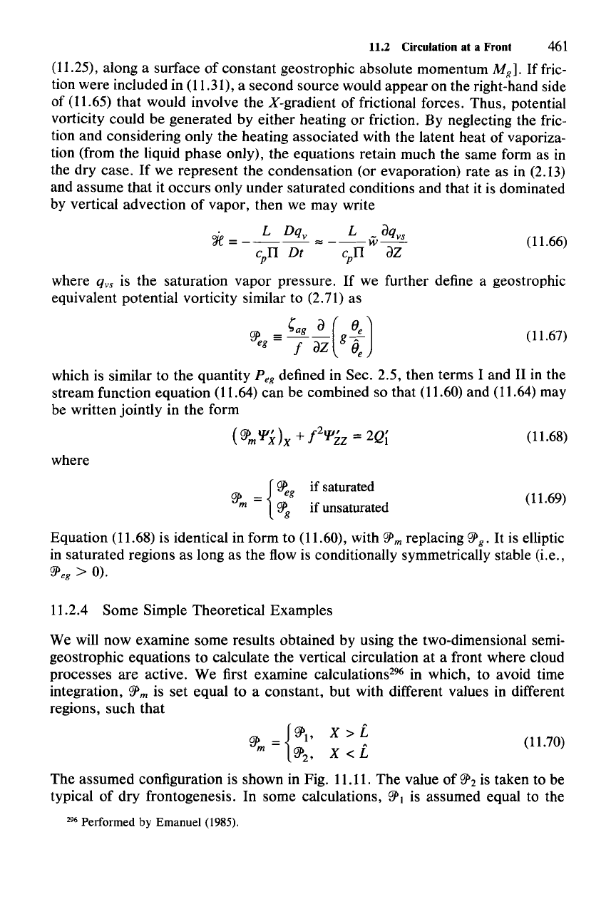
The assumed configuration is shown in Fig. 11.11. The value of

is taken to be

typical of dry frontogenesis. In some calculations,

W'l

is assumed equal to the

296 Performed by

Emanuel

(1985).

462 11 Precipitating Clouds in Extratropical Cyclones

X-

Figure 11.11 Configuration of potential vorticity

'!J'm

used to calculate idealized two-dimensional

circulation at a front. (Adapted from Emanuel, 1985. Reproduced with permission from the American

Meteorological Society.)

value assumed for

rg>2,

and the calculations reduce to the case of dry frontogenesis.

In other calculations,

rg>,

is assigned a value characteristic of cloudy conditions.

rg>,

is assumed to be a small positive value, which assumes that the frontal cloud zone

is characterized by nearly neutral conditional symmetric instability (Sec. 2.9.1).

remains unspecified how the neutral condition is achieved. However, there is

empirical evidence from sounding and aircraft data in frontal zones to support this

assumption.P? According to this parameterization of a frontal-cloud zone,

rg>1

can

be regarded as

rg>

eg in (11.69), while

rg>2

rg>

g »

The calculations with

rg>

m given by (11.70) have been made with the stream

function equation (11.68) for two cases of confluence forcing [defined by term

-ugxb

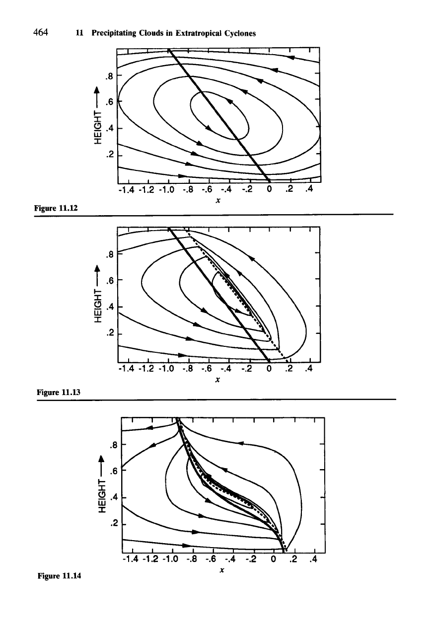
in (11.11) and illustrated in Fig. 11.6]. In the first case, the thermal gradient

is prescribed such that the vertical shear of

implied by thermal-wind balance,

is a constant. The transverse stream functions for the dry and moist versions

this case appear in Fig. 11.12 and 11.13, respectively. The results have been

transformed to physical

(x)

space. The effect of the clouds clearly is to concen-

trate the lifting into a more narrow zone than in the case of dry semigeostrophic

frontogenesis. In a second moist case, whose results are in Fig. 11.14, the vertical

shear of

is specified to decrease with distance X from

The effect of the

horizontal variation

the shear is to give the front a curving shape in the vertical,

with a steeper slope nearer the surface than in the midtroposphere.

Calculations with (11.68)

can

be made less restrictive by allowing the frontal

circulation to develop in time by letting

rg>

m evolve as a result of the condensa-

tional

heating?"

The evolution of the field of potential vorticity

rg>

g is implied by

(11.65) and (11.66). To represent frontal clouds,

rg>

eg is again set equal to a small

positive number, representing that the atmosphere has adjusted to a state of near

conditionally symmetric neutrality. This condition is assumed to apply whenever

297 See Emanuel (1985).

298 This procedure was suggested by Thorpe and Emanuel (1985).

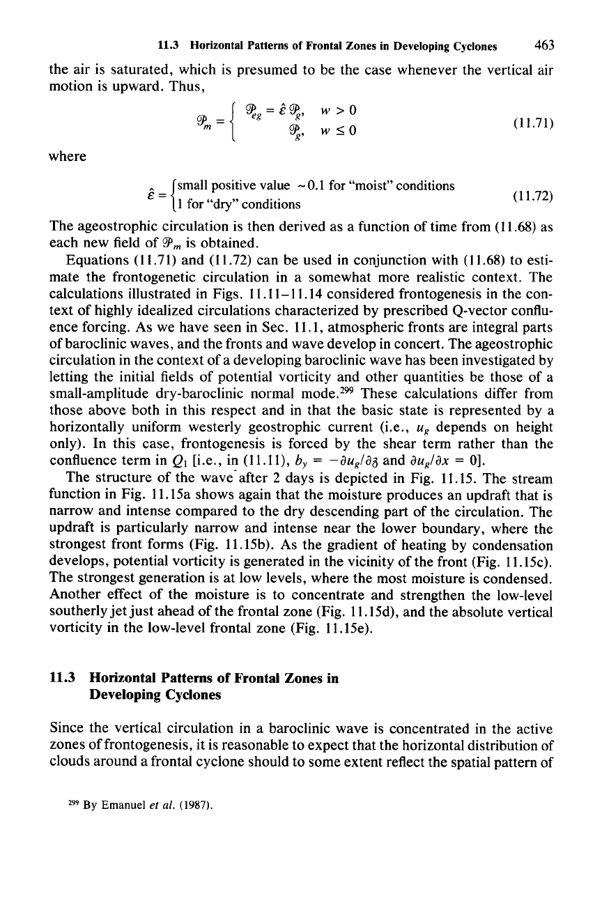
11.3 Horizontal Patterns of Frontal Zones in Developing Cyclones 463

the air is

saturated,

which is

presumed

to be the case whenever the vertical air

motion is upward.

Thus,

where

w > 0

w s 0

(11.71)

A _ {Smallpositive value - 0.1 for "moist" conditions

e (11.72)

- 1 for "dry" conditions

The

ageostrophic circulation is

then

derived as a function

time from (11.68) as

each

new

field

'!Pm

is obtained.

Equations

(11.71) and (11.72)

can

be used in conjunction with (11.68) to esti-

mate

the frontogenetic circulation in a somewhat more realistic context. The

calculations illustrated in Figs. 11.11-11.14 considered frontogenesis in the con-

text

highly idealized circulations characterized by prescribed Q-vector conflu-

ence forcing. As we have seen in Sec. 11.1, atmospheric fronts are integral parts

ofbaroclinic

waves, and the fronts and wave develop in concert. The ageostrophic

circulation in the

context

a developing baroclinic wave has been investigated by

letting the initial fields

potential vorticity and

other

quantities be those

small-amplitude dry-baroclinic normal mode.P? These calculations differ from

those

above

both

in this

respect

and in

that

the basic state is represented by a

horizontally uniform westerly geostrophic current (i.e.,

depends on height

only). In this

case,

frontogenesis is forced by the shear term rather than the

confluence

term

in QI [i.e., in (11.11), by = -auli/aa and

auli/ax

= 0].

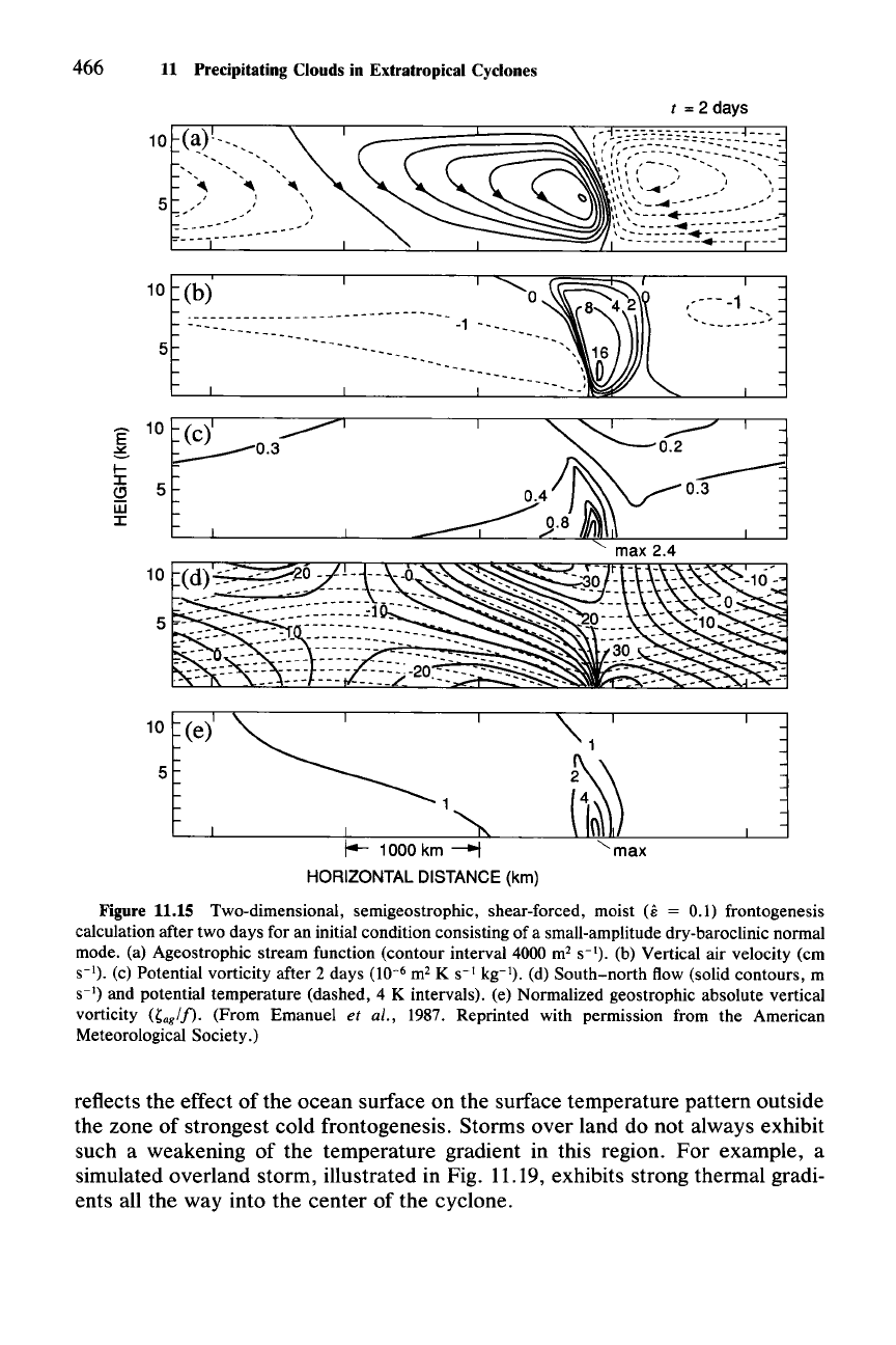
The

structure

the wave- after 2 days is depicted in Fig. 11.15. The stream

function in Fig. 11.15a shows again

that

the moisture produces an updraft that is

narrow

and

intense

compared

to the dry descending part

the circulation. The

updraft is particularly

narrow

and intense near the lower boundary, where the

strongest front forms (Fig. 11.15b). As the gradient

heating by condensation

develops, potential vorticity is generated in the vicinity

the front (Fig. 11.15c).

The

strongest generation is at low levels, where the most moisture is condensed.

Another

effect

the moisture is to

concentrate

and strengthen the low-level

southerly

jet

just

ahead

the frontal zone (Fig. 11.15d), and the absolute vertical

vorticity in

the

low-level frontal zone (Fig. 11.15e).

11.3 Horizontal Patterns of Frontal Zones in

Developing

Cyclones

Since the vertical circulation in a baroclinic wave is concentrated in the active

zones

frontogenesis, it is reasonable to

expect

that

the horizontal distribution of

clouds around a frontal cyclone should to some

extent

reflect the spatial pattern of

299 By Emanuel et al. (1987).

464 11 Precipitating Clouds in Extratropical Cyclones

i .6

~.4

-1.4 -1.2 -1.0 -.8 -.6 -.4 -.2 0 .2 .4

Figure 11.12

i .6

-1.4 -1.2 -1.0 -.8 -.6 -.4 -.2 0 .2 .4

Figure 11.13

i .6

Figure 11.14

-1.4 -1.2 -1.0 -.8 -.6 -.4 -.2 0 .2 .4

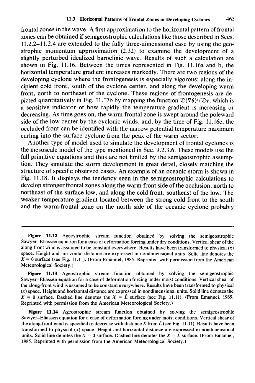
11.3 Horizontal Patterns of Frontal Zones in Developing Cyclones 465

frontal zones in the wave. A first approximation to the horizontal pattern offrontal

zones can be obtained if semigeostrophic calculations like those described in Sees.

11.2.2-11.2.4 are extended to the fully three-dimensional case by using the geo-

strophic momentum approximation (2.32) to examine the development of a

slightly perturbed idealized baroclinic wave. Results of such a calculation are

shown in Fig. 11.16. Between the times represented in Fig. 11.16a and b, the

horizontal temperature gradient increases markedly. There are two regions of the

developing cyclone where the frontogenesis is especially vigorous: along the in-

cipient cold front, south of the cyclone center, and along the developing warm

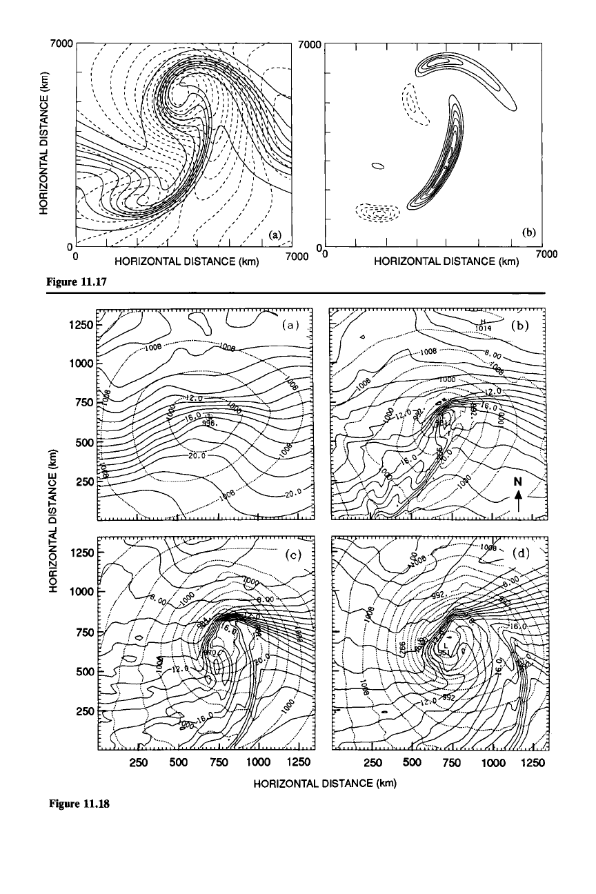
front, north to northeast of the cyclone. These regions of frontogenesis are de-

picted quantitatively in Fig. 11.17b by mapping the function

'JJ(V()2/'JJT, which is

a sensitive indicator of how rapidly the temperature gradient is increasing or

decreasing. As time goes on, the warm-frontal zone is swept around the poleward

side of the low center by the cyclonic winds, and, by the time of Fig. 11.16c, the

occluded front can be identified with the narrow potential temperature maximum

curling into the surface cyclone from the peak of the warm sector.

Another type of model used to simulate the development of frontal cyclones is

the mesoscale model of the type mentioned in Sec. 9.2.3.6. These models use the

full primitive equations and thus are not limited by the semigeostrophic assump-

tion. They simulate the storm development in great detail, closely matching the

structure of specific observed cases. An example of an oceanic storm is shown in

Fig. 11.18.

displays the tendency seen in the semigeostrophic calculations to

develop stronger frontal zones along the warm-front side of the occlusion, north to

northeast of the surface low, and along the cold front, southeast of the low. The

weaker temperature gradient located between the strong cold front to the south

and the warm-frontal zone on the north side of the oceanic cyclone probably

Figure 11.12 Ageostrophic stream function obtained by solving the semigeostrophic

Sawyer-Eliassen equation for a case of deformation forcing under dry conditions. Vertical shear of the

along-front wind is assumed to be constant everywhere. Results have been transformed to physical

(x)

space. Height and horizontal distance are expressed in nondimensional units. Solid line denotes the

X = 0 surface (see Fig. 11.11). (From Emanuel, 1985. Reprinted with permission from the American

Meteorological Society.)

Figure 11.13 Ageostrophic stream function obtained by solving the semigeostrophic

Sawyer-Eliassen equation for a case of deformation forcing under moist conditions. Vertical shear of

the along-front wind is assumed to be constant everywhere. Results have been transformed to physical

(x) space. Height and horizontal distance are expressed in nondimensional units. Solid line denotes the

X = 0 surface. Dashed line denotes the X = t. surface (see Fig. 11.11). (From Emanuel, 1985.

Reprinted with permission from the American Meteorological Society.)

Figure 11.14 Ageostrophic stream function obtained by solving the semigeostrophic

Sawyer-Eliassen equation for a case of deformation forcing under moist conditions. Vertical shear of

the along-front wind is specified to decrease with distance

X from t. (see Fig. 11.11). Results have been

transformed to physical

(x)

space. Height and horizontal distance are expressed in nondimensional

units. Solid line denotes the

X = 0 surface. Dashed line denotes the X = t. surface. (From Emanuel,

1985. Reprinted with permission from the American Meteorological Society.)

466 11 Precipitating Clouds in Extratropical Cyclones

t = 2 days

E 10 (c)

0.3

I-

a 5

::c

---------=

0.3

Figure 11.15 Two-dimensional, sernigeostrophic, shear-forced, moist (e = 0.1) frontogenesis

calculation after two days for an initial condition consisting of a small-amplitude dry-baroclinic normal

mode. (a) Ageostrophic stream function (contour interval 4000 m

S-I). (b) Vertical air velocity (ern

S-I). (c) Potential vorticity after 2 days (10-

K S-I kg-I). (d) South-north flow (solid contours, m

S-I) and potential temperature (dashed, 4 K intervals). (e) Normalized geostrophic absolute vertical

vorticity

(~ag/f).

(From Emanuel et al., 1987. Reprinted with permission from the American

Meteorological Society.)

reflects the effect of the ocean surface on the surface temperature pattern outside

the zone of strongest cold frontogenesis. Storms over land do not always exhibit

such a weakening of the temperature gradient in this region.

For

example, a

simulated overland storm, illustrated in Fig. 11.19, exhibits strong thermal gradi-

ents all the way into the center of the cyclone.

11.4 Clouds and Precipitation in a Frontal Cyclone 467

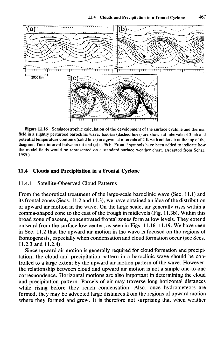
Figure 11.16 Semigeostrophic calculation of the development of the surface cyclone and thermal

field in a slightly perturbed baroclinic wave. Isobars (dashed lines) are shown at intervals of 3 mb and

potential temperature contours (solid lines) are given at intervals of 2 K with colder air at the top of the

diagram. Time interval between (a) and (c) is

96 h. Frontal symbols have been added to indicate how

the model fields would be represented on a standard surface weather chart. (Adapted from Schar,

1989.)

11.4 Clouds and Precipitation in a Frontal Cyclone

11.4.1 Satellite-Observed Cloud Patterns

From the theoretical treatment of the large-scale baroclinic wave (Sec. 11.1) and

its frontal zones (Sees. 11.2 and 11.3), we have obtained an idea of the distribution

of upward air motion in the wave. On the large scale, air generally rises within a

comma-shaped zone to the east

ofthe

trough in midlevels (Fig. 11.3b). Within this

broad zone of ascent, concentrated frontal zones form at low levels. They extend

outward from the surface low center, as seen in Figs. 11.16-11.19. We have seen

in Sec. 11.2 that the upward air motion in the wave is focused on the regions of

frontogenesis, especially when condensation and cloud formation occur (see Sees.

11.2.3 and 11.2.4).

Since upward air motion is generally required for cloud formation and precipi-

tation, the cloud and precipitation pattern in a baroclinic wave should be con-

trolled to a large extent by the upward air motion pattern of the wave. However,

the relationship between cloud and upward air motion is not a simple one-to-one

correspondence. Horizontal motions are also important in determining the cloud

and precipitation pattern. Parcels of air may traverse long horizontal distances

while rising before they reach condensation. Also, once hydrometeors are

formed, they may be advected large distances from the regions of upward motion

where they formed and grew.

is therefore not surprising that when weather

7000

,---.-------.----.----.------.-----...,--,

HORIZONTAL

DISTANCE

(km)

7000

(b)

,-,~~

I 1\'

\\,1\

" ,

, '

--'

7000

(a)

HORIZONTAL

DISTANCE

(km)

7000

(J)

...J

::c

Figure 11.17

;[

(J)

...J

::c

250

500 750

1000 1250

250

500

750 1000

1250

HORIZONTAL

DISTANCE

(km)

Figure 11.18