Heiman G. Basic Statistics for the Behavioral Sciences

Подождите немного. Документ загружается.

108 CHAPTER 5 / Measures of Variability: Range, Variance, and Standard Deviation

27. What is a researcher communicating with each of the following statements?

(a) “The line graph of the means was relatively flat, although the variability in

each condition was quite large.” (b) “For the sample of men ( and )

we conclude...”(c) “We expect that in the population the average score is 14

and the standard deviation is 3.5...”(Chs. 4, 5)

28. For each of the following, identify the conditions of the independent variable, the

dependent variable, their scales of measurement, which measure of central

tendency and variability to compute and which scores you would use in the com-

putations. (a) We test whether participants laugh longer (in seconds) to jokes told

on a sunny or rainy day. (b) We test babies whose mothers were or were not

recently divorced, measuring whether the babies lost weight, gained weight, or

remained the same. (c) We compare a group of adult children of alcoholics to a

group whose parents were not alcoholics. In each, we measure participants’

income. (d) We count the number of creative ideas produced by participants who

are paid either 5, 10, or 50 cents per idea. (e) We measure the number of words in

the vocabulary of 2-year-olds as a function of whether they have 0, 1, 2, or 3 older

siblings. (f) We compare people 5 years after they have graduated from either high

school, a community college, or a four-year college. Considering all participants

at once, we rank order their income. (Chs. 2, 4, 5)

29. For each experiment in question 28, indicate the type of graph you would create,

and how you would label the and axes. (Chs. 2, 4)YX

SD 5 3M 5 14

■ ■ ■ SUMMARY OF

FORMULAS

1. The formula for the range is

Range  highest score  lowest score

2. The computational formula for the sample

variance is

3. The computational formula for the sample

standard deviation is

©X

1©X2

©X

1©X2

4. The computational formula for estimating the

population variance is

5. The computational formula for estimating the

population standard deviation is

©X

1©X2

N 2 1

©X

1©X2

N 2 1

109

z-Scores and the Normal

Curve Model

GETTING STARTED

To understand this chapter, recall the following:

■

From Chapter 3, that relative frequency is the proportion of time that scores

occur, and that it corresponds to the proportion of the area under the normal

curve; that a percentile equals the percent of the area under the curve to the

left of a score.

■

From Chapter 4, that the larger a score’s deviation, the farther into the tail of

the distribution it lies and the lower is its simple frequency and relative frequency.

■

From Chapter 5, that and indicate the “average” deviation of scores

around and , respectively.

Your goals in this chapter are to learn

■

What a z-score is and what it tells you about a raw score’s relative standing.

■

How the standard normal curve is used with z-scores to determine relative

frequency, simple frequency, and percentile.

■

The characteristics of the sampling distribution of means and what the

standard error of the mean is.

■

How computing z-scores for sample means is used to determine their relative

frequency.

X

The techniques discussed in the preceding chapters for graphing, measuring central

tendency, and measuring variability comprise the descriptive procedures used in most

behavioral research. In this chapter, we’ll combine these procedures to answer another

question about data: How does any one particular score compare to the other scores in a

sample or population? We answer this question by transforming raw scores into z-scores.

In the following sections, we discuss (1) the logic of z-scores and their simple com-

putation, (2) how z-scores are used to describe individual scores, and (3) how z-scores

are used to describe sample means.

NEW STATISTICAL NOTATION

Statistics often involve negative and positive numbers. Sometimes, however, we ignore

a number’s sign. The size of a number, regardless of its sign, is the absolute value of

the number. When we do not ignore the sign, you’ll encounter the symbol , which

means “plus or minus.” Saying “ ,” means or . Saying “the scores between

,” means all possible scores from , through 0, up to and including .1121;1

2111;1

;

110 CHAPTER 6 / z-Scores and the Normal Curve Model

BinkySlug

Attractiveness scores

Biff

25 30 35 40 45 50 55 60 65 70 75 80 85 90 95

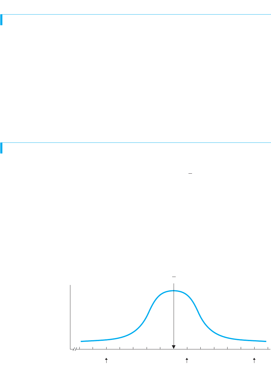
FIGURE 6.1

Frequency distribution of

attractiveness scores at

Prunepit U

Scores for three individuals

are identified on the axis.X

WHY IS IT IMPORTANT TO KNOW ABOUT z-SCORES?

Recall that we transform raw scores to make different variables comparable and to

make scores within the same distribution easier to interpret. The “z-transformation” is

the Rolls-Royce of transformations because with it we can compare and interpret

scores from virtually any normal distribution of interval or ratio scores.

Why do we need to do this? Because researchers usually don’t know how to inter-

pret someone’s raw score: Usually, we won’t know whether, in nature, a score should

be considered high or low, good, bad, or what. Instead, the best we can do is compare a

score to the other scores in the distribution, describing the score’s relative standing.

Relative standing reflects the systematic evaluation of a score relative to the sample or

population in which the score occurs. The way to calculate the relative standing of a

score is to transform it into a z-score. As you’ll see, with z-scores we can easily deter-

mine the underlying raw score’s location in a distribution, its relative and simple

frequency, and its percentile. All of this helps us to know whether the individual’s raw

score was relatively good, bad, or in-between.

UNDERSTANDING z-SCORES

To see how z-scores reflect relative standing, let’s say that we conduct a study at

Prunepit University in which we measure the “attractiveness” of a sample of men. The

scores form the normal curve in Figure 6.1, with a . Of these scores, we espe-

cially want to interpret those of three men: Slug, who scored 35; Binky, who scored 65;

and Biff, who scored 90. Using the statistics you’ve learned, you already know how to

do this. Let’s review.

What would we say to Slug? “Bad news, Slug. Your score places you far below aver-

age in attractiveness. What’s worse, down in the tail, the height of the curve above your

score indicates a low frequency, so not many men received this low score. Also, the pro-

portion of the area under the curve at your score is small, so the relative frequency—

the proportion of all men receiving your score—is low. Finally, Slug, your percentile is

low, so a small percentage scored below you while a large percentage scored above

you. So Slug, scores such as yours are relatively infrequent, and few scores are lower

than yours.”

X 5 60

Understanding z-Scores 111

For Binky, there’s good news and bad news. “The good news, Binky, is that your

score of 65 is above the mean, which is also the median; you are better-looking than

more than 50% of these men. The bad news is that you are not far above the mean.

Also, the area under the curve at your score is relatively large, and thus the relative fre-

quency of equally attractive men is large. What’s worse, a relatively large part of the

distribution has higher scores.”

And then there’s Biff. “Yes, Biff, your score of 90 places you well above average in

attractiveness. In fact, as you have repeatedly told everyone, you are one of the most

attractive men around. Also, the area under the curve at your score is quite small, so

only a small proportion of men are equally attractive. Finally, the area under the curve

to the left of your score is relatively large, so if we cared to figure it out, we’d find that

you are at a very high percentile, with only a small percentage above you.”

These descriptions are based on each man’s relative standing because, considering

our “parking lot” approach to the normal curve, we literally determined where each

stands in the parking lot compared to everyone else. However, there are two problems

with these descriptions. First, they were somewhat subjective and imprecise. Second,

to get them we had to look at all scores in the distribution. However, recall that the

point of statistics is to accurately summarize our data so that we don’t need to look at

every score. The way to obtain the above information, but more precisely and without

looking at every score, is to compute each man’s z-score.

Our description of each man above was based on how far above or below the mean

his raw score appeared to be. To precisely determine this distance, our first calcula-

tion is to determine a score’s deviation, which equals . For example, Biff’s

score of 90 deviates by Likewise, Slug’s score of

35 deviates by . Such deviations sound impressive, but are they?

We have the same problem with deviations that we had with raw scores; we don’t

necessarily know whether a particular deviation should be considered large or small.

However, looking at the distribution, we see that only a few scores deviate by such

large amounts and that is what makes them impressive. Thus, a score is impressive if

it is far from the mean, and “far” is determined by how often other scores deviate

from the mean by that amount.

Therefore, to interpret a score’s location, we need to compare its deviation to all

deviations; we need a standard to compare to each deviation; we need the standard

deviation! As you know, we think of the standard deviation as our way of computing

the “average deviation.” By comparing a score’s deviation to the standard deviation,

we can describe the location of the score in terms of this average deviation. Thus, say

that, the sample standard deviation for the attractiveness scores is 10. Biff’s devia-

tion of is equivalent to 3 standard deviations, so Biff’s raw score is located

3 standard deviations above the mean. Thus, his raw score is impressive because it

is three times as far above the mean as the “average” amount that scores were about

the mean.

By transforming Biff’s deviation into standard deviation units, we have computed

his z-score. A z-score is the distance a raw score is from the mean when measured in

standard deviations. The symbol for a z-score in a sample or population is z.

A z-score always has two components: (1) either a positive or negative sign which

indicates whether the raw score is above or below the mean, and (2) the absolute value

of the z-score which indicates how far the score lies from the mean when measured in

standard deviations. So, Biff is above the mean by 3 standard deviations, so his z-score

is . If he had been below the mean by this amount, he would have .

Thus, like any raw score, a z-score is a location on the distribution. However,

the important part is that a z-score also simultaneously communicates its distance from

z 52313

130

35 2 60 5225

1because 90 2 60 5130.2130

X 2 X

112 CHAPTER 6 / z-Scores and the Normal Curve Model

the mean. By knowing where a score is relative to the mean, we know the score’s rela-

tive standing within the distribution.

REMEMBER A z-score describes a raw score’s location in terms of how far

above or below the mean it is when measured in standard deviations.

Computing z-Scores

Above, we computed Biff’s z-score in two steps. First, we found the score’s deviation

by subtracting the mean from the raw score. Then we divided the score’s deviation by

the standard deviation. So,

The formula for transforming a raw score in a sample

into a z-score is

z 5

X 2 X

(This is both the definitional and the computational formula.) We are computing a

z-score from a sample of scores, so we use the descriptive sample standard deviation,

(the formula with the final division by ). When starting from scratch with a sample

of raw scores, first compute and and then substitute their values into the formula.

To find Biff’s z-score, we substitute his raw score of 90, the of 60, and the of 10

into the formula:

Find the deviation in the numerator first and always subtract from . This gives

After dividing,

Likewise, Binky’s raw score was 65, so

Binky’s raw score is literally one-half of one standard deviation above the mean.

And finally, Slug’s raw score is 35, so

Here, 35 minus 60 results in a deviation of minus 25, so his z-score is 2.50. Slug’s

raw score is 2.5 standard deviations below the mean.

Of course, a raw score that equals the mean produces a z-score of 0, because it is zero

distance from itself. For example, an attractiveness score of 60 will produce an and

that are the same number, so their difference is 0.

z 5

X 2 X

35 2 60

225

522.50

z 5

X 2 X

65 2 60

51.50

z 513.00

z 5

130

z 5

X 2 X

90 2 60

Understanding z-Scores 113

We can also compute a z-score for a score in a population, if we know the population

mean ( ) and the true standard deviation of the population . (We never compute

z-scores using the estimated population standard deviation, ) The logic here is the

same as in the previous formula, but using these symbols gives

1σ

2

The formula for transforming a raw score in a population

into a z-score is

z 5

X 2 

The formula for transforming a z-score in a sample into

a raw score is

X 5 1z21S

21 X

Now the answer indicates how far the raw score lies from the population mean when

measured using the population standard deviation. For example, say that in the popula-

tion of attractiveness scores, and . Biff’s raw score of 90 is again a

, but now this is his location in the population of scores.

Notice that the size of a z-score will depend on both the size of the raw score’s deviation

and the size of the standard deviation. Biff’s deviation of 30 was impressive because the

standard deviation was only 10. If the standard deviation had been 30, then Biff would have

had . Now he is not so impressive because his deviation equals

the “average” deviation, indicating that his raw score is among the more common scores.

Computing a Raw Score When z Is Known

Sometimes we know a z-score and want to find the corresponding raw score. For exam-

ple, say that another man, Bucky, scored . What is his raw score? With

and , his z-score indicates that he is 1 standard deviation above the mean. In

other words, he is10 points above 60, so his raw score is 70. What did we just do? We

multiplied his z-score times and then added the mean.S

5 10

X 5 60z 511

z 5 190 2 602>30 511.00

z 5 190 2 602>10 513.00

5 10 5 60

For Bucky’s z-score of

To check this answer, compute the z-score for the raw score of 70. You should end up

with the z-score you started with: .11

X 5 70

X 5110 1 60

X 5 111211021 60

114 CHAPTER 6 / z-Scores and the Normal Curve Model

Finally, say that Fuzzy has a (with and ). Then his raw

score is

Adding a negative number is the same as subtracting its positive value, so

Fuzzy has a raw score of 47.

The above logic is also used to transform a z-score into its corresponding raw score

in the population. Using the symbols for the population gives

X 5 47

X 5213 1 60

X 5 121.30211021 60

5 10X 5 60z 521.30

The formula for transforming a z-score in a population into

a raw score is

X 5 1z21σ

21 

Here, we multiply the z-score times the population standard deviation and then add . So,

say that Fuzzy is from the population where and . For his z of we

have: He has a raw score of 47 in the population.

After transforming a raw score or z-score, always check whether your answer makes

sense. At the very least, raw scores smaller than the mean must produce negative

z-scores, and raw scores larger than the mean must produce positive z-scores. When

working with z-score, always pay close attention to the positive or negative sign!

Further, as you’ll see, we seldom obtain z-scores greater than or less than .

Although they are possible, be very skeptical if you compute such a z-score, and

double-check your work.

2313

X 5 121.30211021 60 5 47.

21.30σ

5 10 5 60



■

A indicates that the raw score is above the

mean, a that it is below the mean.

■

The absolute value of z indicates the score’s distance

from the mean, measured in standard deviations.

MORE EXAMPLES

In a sample, and To find z for

To find the raw score for

522.15 1 25 5 22.85

X 5 1z21S

21 X 5 12.4321521 25

z 52.43:

z 5

X 2 X

32 2 25

511.40

X 5 32:S

5 5.X 5 25

For Practice

With and ,

1. What is for

2. What produces ?

With and ,

3. What is the for a score of 132?

4. What produces ?

Answers

4. X 5 111.4211621 100 5 122.4

z 5 1132 2 1002>16 512.00

X 5 121.30211021 50 5 37

z 5 144 2 502>10 52.60

z 511.4X

5 16 5 100

z 521.30X

X 5 44?z

5 10X 5 50

A QUICK REVIEW

Interpreting z-Scores Using the z-Distribution 115

Slug Biff

25 30 35 40 45 50 55 60 65 959085807570

–3

–2

–1

0+1

Binky

aw scores

-scores

=10

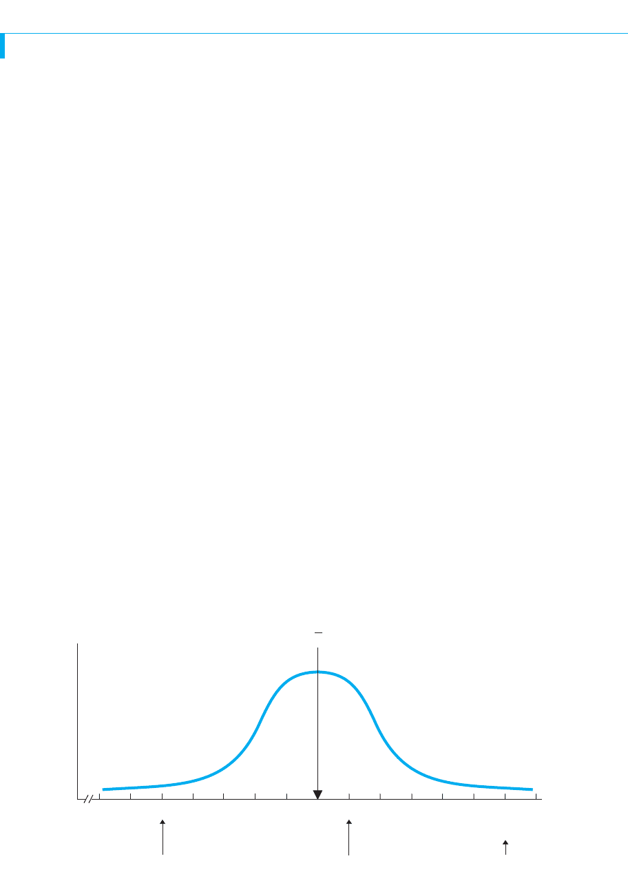
FIGURE 6.2

z-distribution of attractiveness scores at Prunepit U

The labels on the axis show first the raw scores and then the z-scores.X

INTERPRETING z-SCORES USING THE z-DISTRIBUTION

The reason that z-scores are so useful is that they directly communicate the relative

standing of a raw score. The way to see this is to first envision any sample or popula-

tion as a z-distribution. A z-distribution is the distribution produced by transforming

all raw scores in the data into z-scores. For example, say that our attractiveness scores

produce the z-distribution shown in Figure 6.2. The axis is also labeled using the

original raw scores to show that by creating a z-distribution, we only change the way

that we identify each score. Saying that Biff has a z of is merely another way to

say that he has a raw score of 90. He is still at the same point on the distribution, so

Biff’s z of has the same frequency, relative frequency, and percentile as his raw

score of 90.

By envisioning such a z-distribution, you can see how z-scores form a standard way

to communicate relative standing. The z-score of 0 indicates that the raw score equals

the mean. A “ ” indicates that the z-score (and raw score) is above and graphed to the

right of the mean. Positive z-scores become increasingly larger as we proceed farther

to the right. Larger positive z-scores (and their corresponding raw scores) occur less

frequently. Conversely, a “ ” indicates that the z-score (and raw score) is below and

graphed to the left of the mean. Negative z-scores become increasingly larger as we

proceed farther to the left. Larger negative z-scores (and their corresponding raw

scores) occur less frequently. However, as shown, most of the z-scores are between

and .

Do not be misled by negative z-scores: A raw score that is farther below the mean is

a smaller raw score, but it produces a negative z-score whose absolute value is larger.

Thus, for example, a z-score of corresponds to a lower raw score than a z-score of

Also, a negative z-score is not automatically a bad score. For some variables, the

goal is to have as low a raw score as possible (for example, errors on a test). With these

variables, larger negative z-scores are best.

21.

2313

116 CHAPTER 6 / z-Scores and the Normal Curve Model

REMEMBER On a normal distribution, the larger the z-score, whether posi-

tive or negative, the farther the raw score is from the mean and the less fre-

quently the raw score and the z-score occur.

Figure 6.2 illustrates three important characteristics of any z-distribution.

1. A z-distribution has the same shape as the raw score distribution. Only when the

underlying raw score distribution is normal will its z-distribution be normal.

2. The mean of any z-distribution is 0. Whatever the mean of the raw scores is, it

transforms into a z-score of 0.

3. The standard deviation of any z-distribution is 1. Whether the standard deviation

in the raw scores is 10 or 100, it is still one standard deviation, which transforms

into an amount in z-scores of 1.

Now you can see why z-scores are so useful: All normal z-distributions are similar,

so a particular z-score will convey the same information in every distribution. There-

fore, the way to interpret the individual scores from any normally distributed variable

is to envision a z-distribution similar to Figure 6.2. Then, for example, if we know that

z is 0, we know that the corresponding raw score is at the mean (and at the median and

mode). Also, recall from Chapter 5 that the two raw scores that are from the

mean delineate the middle 68% of the curve. Now you know that being from the

mean produces z-scores of . Therefore, approximately 68% of the scores on any nor-

mal distribution will be between the z-scores at . Likewise, any other z-score will

always be in the same relative location, so if z is , then, like Binky’s, the raw score

is slightly above the mean and slightly above the 50th percentile, where scores still

have a high simple and relative frequency. But, if z is , then, like Biff’s, the raw

score is one of the highest possible scores in the upper tail of the distribution, having a

low frequency, a low relative frequency and a very high percentile. And so on.

REMEMBER The way to interpret the raw scores in any sample or population

is to determine their relative standing by envisioning them as a z-distribution.

As you’ll see in the following sections, in addition to describing relative standing as

above, z distributions have two additional uses: (1) comparing scores from different

distributions and (2) computing the relative frequency of scores.

USING z-SCORES TO COMPARE DIFFERENT VARIABLES

An important use of z-scores is when we compare scores from different variables.

Here’s a new example. Say that Cleo received a grade of 38 on her statistics quiz and

a grade of 45 on her English paper. These scores reflect different kinds of tasks, so

it’s like comparing apples to oranges. The solution is to transform the raw scores

from each class into z-scores. Then we can compare Cleo’s relative standing in

English to her relative standing in statistics, so we are no longer comparing apples

and oranges.

Note: The z-transformation equates or standardizes different distributions, so

z-scores are often referred to as standard scores.

Say that for the statistics quiz the was 30 and the was 5. Cleo’s grade of

38 becomes . For the English paper, the was 40 and the was 10, so her

45 becomes A z-score of is farther above any mean than a z-score of11.6z 51.5.

Xz 511.6

1.50

;1S

Using z-Scores to Determine the Relative Frequency of Raw Scores 117

English

Statistics

–3

–2

–1

Attila in

Statistics,

z = –2

Attila in

English,

z = –1

Cleo in

English,

z = +.5

Cleo in

Statistics,

z = +1.6

z-scores

Statistics

English

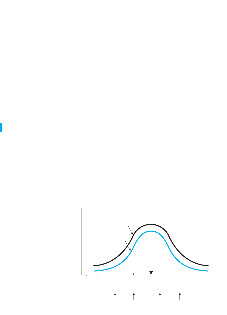
FIGURE 6.3

Comparison of distribu-

tions for statistics and

English grades, plotted

on the same set of axes

Thus, Cleo did relatively better in statistics because she is farther above the

statistics mean than she is above the English mean.

Another student, Attila, obtained raw scores that produced in statistics and

in English. In which class did he do better? His z-score of in English is rel-

atively better, because it is less distance below the mean.

We can also see these results in Figure 6.3, in which the z-distributions from both

classes are plotted on one set of axes. (The greater height of the English distribution

reflects a larger , with a higher f for each score.) Notice that the raw scores from each

class are spaced differently along the axis, because the classes have different stan-

dard deviations. However, z-scores always increment by one standard deviation,

whether it equals 5 points in statistics or 10 points in English. Therefore, the spacing of

the z-scores is the same for the two classes and so they are comparable. Now we can

see that Cleo scored better in statistics than in English but that Attila scored better in

English than in statistics.

REMEMBER To compare raw scores from two different variables, transform

the scores into z-scores.

USING z-SCORES TO DETERMINE THE RELATIVE FREQUENCY OF RAW SCORES

A third important use of z-scores is for computing the relative frequency of raw scores.

Recall that relative frequency is the proportion of time that a score occurs, and that rel-

ative frequency can be computed using the proportion of the total area under the curve.

We can use the z-distribution to determine relative frequency because, as we’ve seen,

when raw scores produce the same z-score they are at the same location on their distri-

butions. By being at the same location, a z-score delineates the same proportion of the

curve, cutting off the same “slice” of the distribution every time. Thus, the relative fre-

quency at particular z-scores will be the same on all normal z-distributions.

For example, 50% of the raw scores on a normal curve are to the left of the mean,

and scores to the left of the mean produce negative z-scores. In other words, the

21z 521

z 522

z 51.5.