Heiman G. Basic Statistics for the Behavioral Sciences

Подождите немного. Документ загружается.

88 CHAPTER 5 / Measures of Variability: Range, Variance, and Standard Deviation

example, if the grades in a statistics class form a normal distribution with a mean of 80,

then you know that most of the scores are around 80. But are most scores between 79

and 81 or between 60 and 100? By showing how spread out scores are from the mean,

the variance and standard deviation define “around.”

REMEMBER The variance and standard deviation are two measures of vari-

ability that indicate how much the scores are spread out around the mean.

Mathematically, the distance between a score and the mean is the difference between

them. Recall from Chapter 4 that this difference is symbolized by , which is the

amount that a score deviates from the mean. Thus, a score’s deviation indicates how far

it is spread out from the mean. Of course, some scores will deviate by more than oth-

ers, so it makes sense to compute something like the average amount the scores deviate

from the mean. Let’s call this the “average of the deviations.” The larger the average of

the deviations, the greater the variability.

To compute an average, we sum the scores and divide by N. We might find the aver-

age of the deviations by first computing for each participant and then summing

these deviations to find . Finally, we’d divide by N, the number of deviations.

Altogether, the formula for the average of the deviations would be

Average of the deviations

We might compute the average of the deviations using this formula, except for a big

problem. Recall that the sum of the deviations around the mean, , always

equals zero because the positive deviations cancel out the negative deviations. This

means that the numerator in the above formula will always be zero, so the average of

the deviations will always be zero. So much for the average of the deviations!

But remember our purpose here:We want a statistic like the average of the deviations

so that we know the average amount the scores are spread out around the mean. But,

because the average of the deviations is always zero, we calculate slightly more com-

plicated statistics called the variance and standard deviation. Think of them, however,

as each producing a number that indicates something like the average or typical amount

that the scores differ from the mean.

REMEMBER Interpret the variance and standard deviation as roughly indicat-

ing the average amount the raw scores deviate from the mean.

The Sample Variance

If the problem with the average of the deviations is that the positive and negative devia-

tions cancel out, then a solution is to square each deviation. This removes all negative

signs, so the sum of the squared deviations is not necessarily zero and neither is the av-

erage squared deviation.

By finding the average squared deviation, we compute the variance. The sample

variance is the average of the squared deviations of scores around the sample mean.

The symbol for the sample variance is . Always include the squared sign because it

is part of the symbol. The capital S indicates that we are describing a sample, and the

subscript indicates that it is computed for a sample of scores.XX

Σ1X 2 X2

Σ1X 2 X

X 2 X

X – X

In advanced statistics there is a very real statistic called the “average deviation.” This isn’t it.

REMEMBER The symbol stands for the variance in a sample of scores.

The formula for the variance is similar to the previous formula for the average deviation

except that we add the squared sign. The definitional formula for the sample variance is

Although we will see a better, computational formula later, we will use this one now

so that you understand the variance. Say that we measure the ages of some children, as

shown in Table 5.2. The mean age is 5 so we first compute each deviation by subtract-

ing this mean from each score. Next, we square each deviation. Then adding the

squared deviations gives , which here is 28. The N is 7, so

Thus, in this sample, the variance equals 4. In other words, the average squared devia-

tion of the age scores around the mean is 4.

The good news is that the variance is a legitimate measure of variability. The bad news,

however, is that the variance does not make much sense as the “average deviation.” There

are two problems. First, squaring the deviations makes them very large, so the variance is

unrealistically large. To say that our age scores differ from their mean by an average of 4

is silly because not one score actually deviates from the mean by this much. The second

problem is that variance is rather bizarre because it measures in squared units. We meas-

ured ages, so the scores deviate from the mean by 4 squared years (whatever that means!).

Thus, it is difficult to interpret the variance as the “average of the deviations.” The vari-

ance is not a waste of time, however, because it is used extensively in statistics. Also, vari-

ance does communicate the relative variability of scores. If one sample has and

another has , you know that the second sample is more variable because it has a

larger average squared deviation. Thus, think of variance as a number that generally com-

municates how variable the scores are:The larger the variance, the more the scores are

spread out.

The measure of variability that more directly communicates the “average of the de-

viations” is the standard deviation.

The Sample Standard Deviation

The sample variance is always an unrealistically large number because we square each

deviation. To solve this problem, we take the square root of the variance. The answer is

called the standard deviation. The sample standard deviation is the square root of the

5 3

5 1

Σ1X 2 X

5 4

Σ1X 2 X

Σ1X 2 X2

Understanding the Variance and Standard Deviation 89

Participant Age Score – 

12–5 –3 9

23–5 –2 4

34–5 –1 1

45–5 00

56–5 11

67–5 24

78–5 39

N 7 Σ1X 2 X

5 285

1X 2 X

1X 2 X2X

TABLE 5.2

Calculation of Variance

Using the Definitional

Formula

90 CHAPTER 5 / Measures of Variability: Range, Variance, and Standard Deviation

sample variance. (Technically, the standard deviation equals the square root of the av-

erage squared deviation! But that’s why we’ll think of it as somewhat like the “average

deviation”.) Conversely, squaring the standard deviation produces the variance.

The symbol for the sample standard deviation is (which is the square root of the

symbol for the sample variance: ).

REMEMBER The symbol stands for the sample standard deviation.

To create the definitional formula here, we simply add the square root sign to the pre-

vious defining formula for variance. The definitional formula for the sample standard

deviation is

The formula shows that to compute S

we first compute everything inside the square

root sign to get the variance. In our previous age scores the variance was 4. Then we

find the square root of the variance to get the standard deviation. In this case,

The standard deviation of the age scores is 2.

The standard deviation is as close as we come to the “average of the deviations,” and

there are three related ways to interpret it. First, our of 2 indicates that the age scores

differ from the mean by an “average” of 2. Some scores deviate by more and some by

less, but overall the scores deviate from the mean by close to an average of 2. Further,

the standard deviation measures in the same units as the raw scores, so the scores differ

from the mean age by an “average” of 2 years.

Second, the standard deviation allows us to gauge how consistently close together

the scores are and, correspondingly, how accurately they are summarized by the mean.

If is relatively large, then we know that a large proportion of scores are relatively far

from the mean. If is small, then more of the scores are close to the mean, and rela-

tively few are far from it.

And third, the standard deviation indicates how much the scores below the mean de-

viate from it and how much the scores above the mean deviate from it, so the standard

deviation indicates how much the scores are spread out around the mean. To see this,

we find the scores at “plus 1 standard deviation from the mean” and “minus 1

standard deviation from the mean” . For example, our age scores of 2, 3, 4, 5, 6,

7, and 8 produced and , The score that is from the mean is the score

at , or 7. The score that is from the mean is the score at , or 3. Looking

at the individual scores, you can see that it is accurate to say that the majority of the

scores are between 3 and 7.

REMEMBER The standard deviation indicates the “average deviation” from

the mean, the consistency in the scores, and how far scores are spread out

around the mean.

In fact, the standard deviation is mathematically related to the normal curve so that

computing the scores at and is especially useful. For example, say that in11S

–1S

5 – 2–1S

5 1 2

11S

5 2X 5 5

1–1S

111S

5 2

5 14

Σ1X 2 X2

5 S

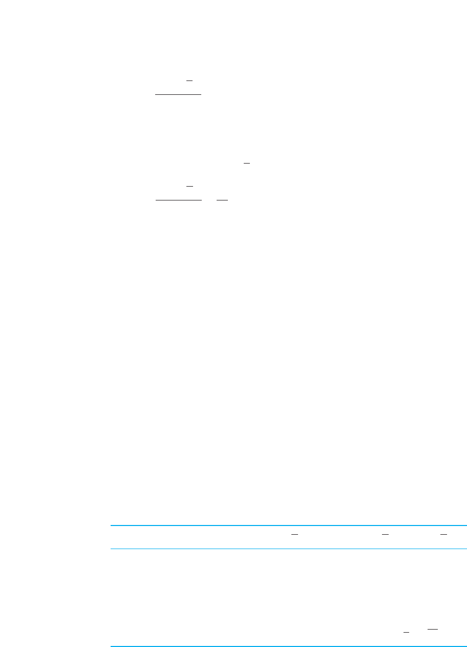
the statistics class with a mean of 80, the is 5. The score at is 75,

and the score at is 85. Figure 5.2 shows about where these scores are

located on a normal distribution.

(Here is how to visually locate about where the scores at and are on any

normal curve. Above the scores close to the mean, the curve forms a downward convex

shape . As you travel toward each tail, the curve changes its pattern to an upward

convex shape The points at which the curve changes its shape are called inflection

points. The scores under the inflection points are the scores that are 1 standard devia-

tion away from the mean.)

Now here’s the important part: These inflection points produce the characteristic bell

shape of the normal curve so that about 34% of the area under the curve is always be-

tween the mean and the score that is at an inflection point. Recall that area under the

curve translates into the relative frequency of scores. Therefore, about 34% of the

scores in a normal distribution are between the mean and the score that is 1 standard

deviation from the mean. Thus, in Figure 5.2, approximately 34% of the scores are be-

tween 75 and 80, and 34% of the scores are between 80 and 85. Altogether, about 68%

of the scores are between the scores at and from the mean. Thus, 68% of

the statistics class has scores between 75 and 85. Conversely, about 16% of the scores

are in the tail below 75, and 16% are above 85. Thus, saying that most scores are be-

tween 75 and 85 is an accurate summary because the majority of scores (68%) are here.

REMEMBER Approximately 34% of the scores in a normal distribution are

between the mean and the score that is 1 standard deviation from the mean.

In summary, here is how the standard deviation (and variance) add to our description

of a distribution. If we know that data form a normal distribution and that, for example,

the mean is 50, then we know where the center of the distribution is and what the typi-

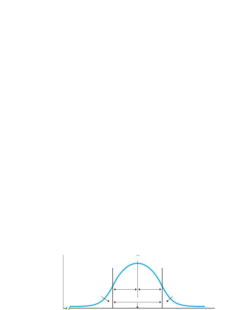
cal score is. With the variability, we can envision the distribution. For example, Figure

5.3 shows the three curves you saw at the beginning of this chapter. Say that I tell you

that is 4. This indicates that participants who did not score 50 missed it by an “aver-

age” of 4 and that most (68%) of the scores fall in the relatively narrow range between

46 and . Therefore, you should envision something like Distribu-

tion A:The high-frequency raw scores are bunched close to the mean, and the middle

68% of the curve is the narrow slice between 46 and 54. If, however, is 7, you know

that the scores are more inconsistent because participants missed 50 by an “average” of

7, and 68% of the scores fall in the wider range between 43 to 57. Therefore, you’d en-

vision Distribution B: A larger average deviation is produced when scores further above

54 150 1 42150 2 42

21S

11S

1´2

1>2

11S

–1S

80 – 5 1at 11S

80 – 5 1at 2 1S

Understanding the Variance and Standard Deviation 91

FIGURE 5.2

Normal distribution

showing scores at plus

or minus 1 standard

deviation

With , the score of 75

is at , and the score of

85 is at . The percent-

ages are the approximate

percentages of the scores

falling into each portion of

the distribution.

11S

–1S

5 5

34% 34%

68%

16%

75 80 85

– 1S

+1S

92 CHAPTER 5 / Measures of Variability: Range, Variance, and Standard Deviation

or below the mean have higher frequency, so the high-frequency part of the distribution

is now spread out between 43 and 57. Lastly, say that is 12; you know that large/-

frequent differences occur, with participants missing 50 by an “average” of 12 points,

so 68% of the scores are between 38 and 62. Therefore, envision Distribution C: Scores

frequently occur that are way above or below 50, so the middle 68% of the distribution

is relatively wide and spread out between 38 and 62.

FIGURE 5.3

Three variations of the normal curve

Scores

Distribution A

Distribution B

Scores

Distribution C

30 35 40 45 50 55 60 65 70

S = 4

030354045505560657075

0 3035404550556065707525

S = 7

S = 12

–S

A QUICK REVIEW

■

The sample variance and the sample standard

deviation are the two statistics to use with the

mean to describe variability.

■

The standard deviation is interpreted as the average

amount that scores deviate from the mean.

MORE EXAMPLES

For the the scores 5, 6, 7, 8, 9, the 7. The vari-

ance is the average squared deviation of the

scores around the mean (here, ). The standard

deviation is the square root of the variance. is in-

terpreted as the average deviation of the scores: Here,

, so when participants missed the mean,

they were above or below 7 by an “average” of 1.41.

Further, in a normal distribution, about 34% of the

scores would be between the and .

About 34% of the scores would be between the and

For Practice

1. The symbol for the sample variance is ____.

2. The symbol for the sample standard deviation

is ____.

5.59 17 2 1.412

8.41 17 1 1.412X

5 1.41

5 2

X 5

3. What is the difference between computing the

standard deviation and the variance?

4. In sample A, ; in sample B, .

Sample A is

____

(more/less) variable and most

scores tend to be

____

(closer to/farther from) the

mean.

5. If and , then 68% of the scores fall

between

____

and

____

Answers

3. The standard deviation is the square root of the variance.

4. less; closer

5. 8; 12

5 2X 5 10

5 11.41S

5 6.82

Use this formula only when describing a sample. It says to first find , then square

that sum, and then divide by N. Subtract that result from . Finally, divide by N again.

For example, for our age scores in Table 5.3, the is 35, is 203, and N is 7.

Putting these quantities in the formula, we have

The squared sum of is , which is 1225, so

Now, 1225 divided by 7 equals 175, so

Because 203 minus 175 equals 28, we have

Finally, after dividing, we have

Thus, again, the sample variance for these age scores is 4.

Do not read any further until you can work this formula!

5 4

203 2 175

203 2

1225

ΣX

1ΣX2

203 2

1352

ΣX

©X

Computing the Sample Variance and Sample Standard Deviation 93

COMPUTING THE SAMPLE VARIANCE AND SAMPLE STANDARD DEVIATION

The previous definitional formulas for the variance and standard deviation are impor-

tant because they show that the core computation is to measure how far the raw scores

are from the mean. However, by reworking them, we have less obvious but faster com-

putational formulas.

Computing the Sample Variance

The computational formula for the sample variance is derived from its previous defini-

tional formula: we’ve replaced the symbol for the mean with its formula and then re-

duced the components.

The computational formula for the sample variance is

ΣX

1ΣX2

Score

416

525

636

749

864

 35  203 ΣX

ΣX

TABLE 5.3

Calculation of Variance

Using the Computational

Formula

94 CHAPTER 5 / Measures of Variability: Range, Variance, and Standard Deviation

Computing the Sample Standard Deviation

The computational formula for the standard deviation merely adds the square root sym-

bol to the previous formula for the variance.

The computational formula for the sample standard deviation is

ΣX

1ΣX2

Use this formula only when computing the sample standard deviation. For example, for

the age scores in Table 5.3, we saw that is 35, is 203, and N is 7. Thus,

As we saw, the computations inside the square root symbol produce the variance,

which is 4, so we have

After finding the square root, the standard deviation of the age scores is

Finally, be sure that your answer makes sense when computing (and ). First,

variability cannot be a negative number because you are measuring the distance scores

are from the mean, and the formulas involve squaring each deviation. Second, watch

for answers that don’t fit the data. For example, if the scores range from 0 to 50, the

mean should be around 25. Then the largest deviation is about 25, so the “average” de-

viation will be much less than 25. However, it is also unlikely that is something like

.80: If there are only two deviations of 25, imagine how many tiny deviations it would

take for the average to be only .80.

Strange answers may be correct for strange distributions, but always check whether

they seem sensible. A rule of thumb is

For any roughly normal distribution, the standard deviation should equal

about one-sixth of the range.

5 2

5 24

203 2

1352

ΣX

A QUICK REVIEW

■

indicates to find the sum of the squared Xs.

■

indicates to find the squared sum of X.

MORE EXAMPLES

For the scores 5, 6, 7, 8, 9:

1ΣX2

ΣX

1. To find the variance,

continued

N 5 5

ΣX

5 5

1 6

1 7

1 8

1 9

5 255

ΣX 5 5 1 6 1 7 1 8 1 9 5 35

Mathematical Constants and the Standard Deviation

As discussed in Chapter 4, sometimes we transform scores by either adding, subtracting,

multiplying, or dividing by a constant. What effects do such transformations have on the

standard deviation and variance? The answer depends on whether we add (subtracting is

adding a negative number) or multiply (dividing is multiplying by a fraction).

Adding a constant to all scores merely shifts the entire distribution to higher or lower

scores. We do not alter the relative position of any score, so we do not alter the spread in

the data. For example, take the scores 4, 5, 6, 7, and 8. The mean is 6. Now add the con-

stant 10. The resulting scores of 14, 15, 16, 17, and 18 have a mean of 16. Before the

transformation, the score of 4 was 2 points away from the mean of 6. In the transformed

data, the score is now 14, but it is still 2 points away from the new mean of 16. In the

same way, each score’s distance from the mean is unchanged, so the standard deviation

is unchanged. If the standard deviation is unchanged, the variance is also unchanged.

Multiplying by a constant, however, does alter the relative positions of scores and

therefore changes the variability. If we multiply the scores 4, 5, 6, 7, and 8 by 10, they

become 40, 50, 60, 70, and 80. The original scores that were 1 and 2 points from the

mean of 6 are now 10 and 20 points from the new mean of 60. Each transformed score

produces a deviation that is 10 times the original deviation, so the new standard devia-

tion is also 10 times greater. (Note that this rule does not apply to the variance. The new

variance will equal the square of the new standard deviation.)

REMEMBER Adding or subtracting a constant does not alter the variability of

scores, but multiplying or dividing by a constant does alter the variability.

THE POPULATION VARIANCE AND THE POPULATION STANDARD DEVIATION

Recall that our ultimate goal is to describe the population of scores. Sometimes re-

searchers will have access to a population of scores, and then they directly calculate

The Population Variance and the Population Standard Deviation 95

2. To find the standard deviation, perform the above

steps and then find the square root, so

5 22.00

5 1.41

ΣX

–

1ΣX2

255 2

1225

5 2.00

225 2 245

255 2

1225

ΣX

1ΣX2

255 2

1352

For Practice

For the scores 2, 4, 5, 6, 6, 7:

1. What is ?

2. What is ?

3. What is the variance?

4. What is the standard deviation?

Answers

4. S

5 22.667 5 1.63

166 –

900

5 2.667

1 4

1 5

1 6

1 7

5 166

1302

5 900

ΣX

1ΣX2

96 CHAPTER 5 / Measures of Variability: Range, Variance, and Standard Deviation

the actual population variance and standard deviation. The symbol for the known and

true population standard deviation is (the is the lowercase Greek letter s,

called sigma). Because the squared standard deviation is the variance, the symbol for

the true population variance is . (In each case, the subscript indicates a popula-

tion of scores.)

The definitional formulas for and are similar to those we saw for a sample:

Population Standard Deviation Population Variance

The only novelty here is that we determine how far each score deviates from the popu-

lation mean, . Otherwise the population standard deviation and variance tell us ex-

actly the same things about the population that we saw previously for a sample: Both

are ways of measuring how much, “on average,” the scores differ from , indicating

how much the scores are spread out in the population. And again, 34% of the popula-

tion will have scores between and the score that is above , and another 34%

will have scores between and the score that is below , for a total of 68%

falling between these two scores.

REMEMBER The symbols and are used when describing the known

true population variability.

The previous defining formulas are important for showing you what and are.

We won’t bother with their computing formulas, because these symbols will appear for

you only as a given, when much previous research allows us to know their values.

However, at other times, we will not know the variability in the population. Then we

will estimate it using a sample.

Estimating the Population Variance and Population

Standard Deviation

We use the variability in a sample to estimate the variability that we would find if we

could measure the population. However, we do not use the previous formulas for the

sample variance and standard deviation as the basis for this estimate. These statistics

(and the symbols and ) are used only to describe the variability in a sample. They

are not for estimating the corresponding population parameters.

To understand why this is true, say that we measure an entire population of scores

and compute its true variance. We then draw many samples from the population and

compute the sample variance of each. Sometimes a sample will not perfectly represent

the population so that the sample variance will be either smaller or larger than the pop-

ulation variance. The problem is that, over many samples, more often than not the sam-

ple variance will underestimate the population variance. The same thing occurs when

using the standard deviation.

In statistical terminology, the formulas for and are called the biased estima-

tors: They are biased toward underestimating the true population parameters. This is

a problem because, as we saw in the previous chapter, if we cannot be accurate, we at

least want our under- and overestimates to cancel out over the long run. (Remember

the statisticians shooting targets?) With the biased estimators, the under- and over-

estimates do not cancel out. Instead, they are too often too small to use as estimates of

the population.

–1σ



11σ



Σ1X 2 2

Xσ

σσ

The sample variance and the sample standard deviation are perfectly ac-

curate for describing a sample, but their formulas are not designed for estimating

the population. To accurately estimate a population, we should have a sample of ran-

dom scores, so here we need a sample of random deviations. Yet, when we measure

the variability of a sample, we use the mean as our reference point, so we encounter

the restriction that the sum of the deviations must equal zero. Because of this, not

all deviations in the sample are “free” to be random and to reflect the variability

found in the population. For example, say that the mean of five scores is 6 and that four

of the scores are 1, 5, 7, and 9. Their deviations are , , 1, and 3, so the sum

of their deviations is . Therefore, the final score must be 8, because it must have a

deviation of 2 so that the sum of all deviations is zero. Thus, the deviation for this

score is determined by the other scores and is not a random deviation that reflects

the variability found in the population. Instead, only the deviations produced by the

four scores of 1, 5, 7, and 9 reflect the variability found in the population. The same

would be true for any four of the five scores. Thus, in general, out of the N scores in

a sample, only N  1 of them (the N of the sample minus 1) actually reflect the vari-

ability in the population.

The problem with the biased estimators ( and ) is that these formulas divide by

. Because we divide by too large a number, the answer tends to be too small. Instead,

we should divide by  1. By doing so, we compute the unbiased estimators of the

population variance and standard deviation. The definitional formulas for the unbiased

estimators of the population variance and standard deviation are

Estimated Population Variance Estimated Population Standard Deviation

Notice we can call them the estimated population standard deviation and the esti-

mated population variance. These formulas are almost the same as the previous

defining formulas that we used with samples: The standard deviation is again the

square root of the variance, and in both the core computation is to determine the

amount each score deviates from the mean and then compute something like an “aver-

age” deviation. The only novelty here is that, when calculating the estimated popula-

tion standard deviation or variance, the final division involves .

The symbol for the unbiased estimator of the standard deviation is the lowercase ,

and the symbol for the unbiased estimator of the variance is the lowercase . To keep

all of your symbols straight, remember that the symbols for the sample involve the cap-

ital or big , and in those formulas you divide by the “big” value of . The symbols for

estimates of the population involve the lowercase or small s, and here you divide by the

smaller quantity,  1. Further, the small is used to estimate the small Greek called

. Finally, think of and as the inferential variance and the inferential standard de-

viation, because the only time you use them is to infer the variance or standard devia-

tion of the population based on a sample. Think of and as the descriptive variance

and standard deviation because they are used to describe the sample.

REMEMBER and describe the variability in a sample; and esti-

mate the variability in the population.

For future reference, the quantity is called the degrees of freedom. The degrees

of freedom is the number of scores in a sample that are free to reflect the variability in

the population. The symbol for degrees of freedom is df, so here .df 5 N – 1

N – 1

ssN

N – 1

Σ1X – X2

N – 1

Σ1X – X2

N – 1

2125

21S

The Population Variance and the Population Standard Deviation 97