Heiman G. Basic Statistics for the Behavioral Sciences

Подождите немного. Документ загружается.

78 CHAPTER 4 / Measures of Central Tendency: The Mean, Median, and Mode

Inferring the Relationship in the Population

Previously we summarized the results of our list-learning experiment in terms of the sam-

ple data. But this is only part of the story. The big question remains: Do these data reflect

a law of nature? Do longer lists produce more recall errors for everyone in the population?

Recall that to make inferences about the population, we must first compute the appro-

priate inferential statistics. Assuming that our data passed the inferential test, we can

conclude that each sample mean represents the population mean that would be found for

that condition. The mean for the 5-item condition was 3, so we infer that if everyone

in the population recalled a 5-item list, the mean error score would be 3. Similarly,

if the population recalled a 10-item list, would equal the condition’s mean of 6, and if

the population recalled a 15-item list, would be 9. Because we are describing how the

scores change in the population, we are describing the relationship in the population.

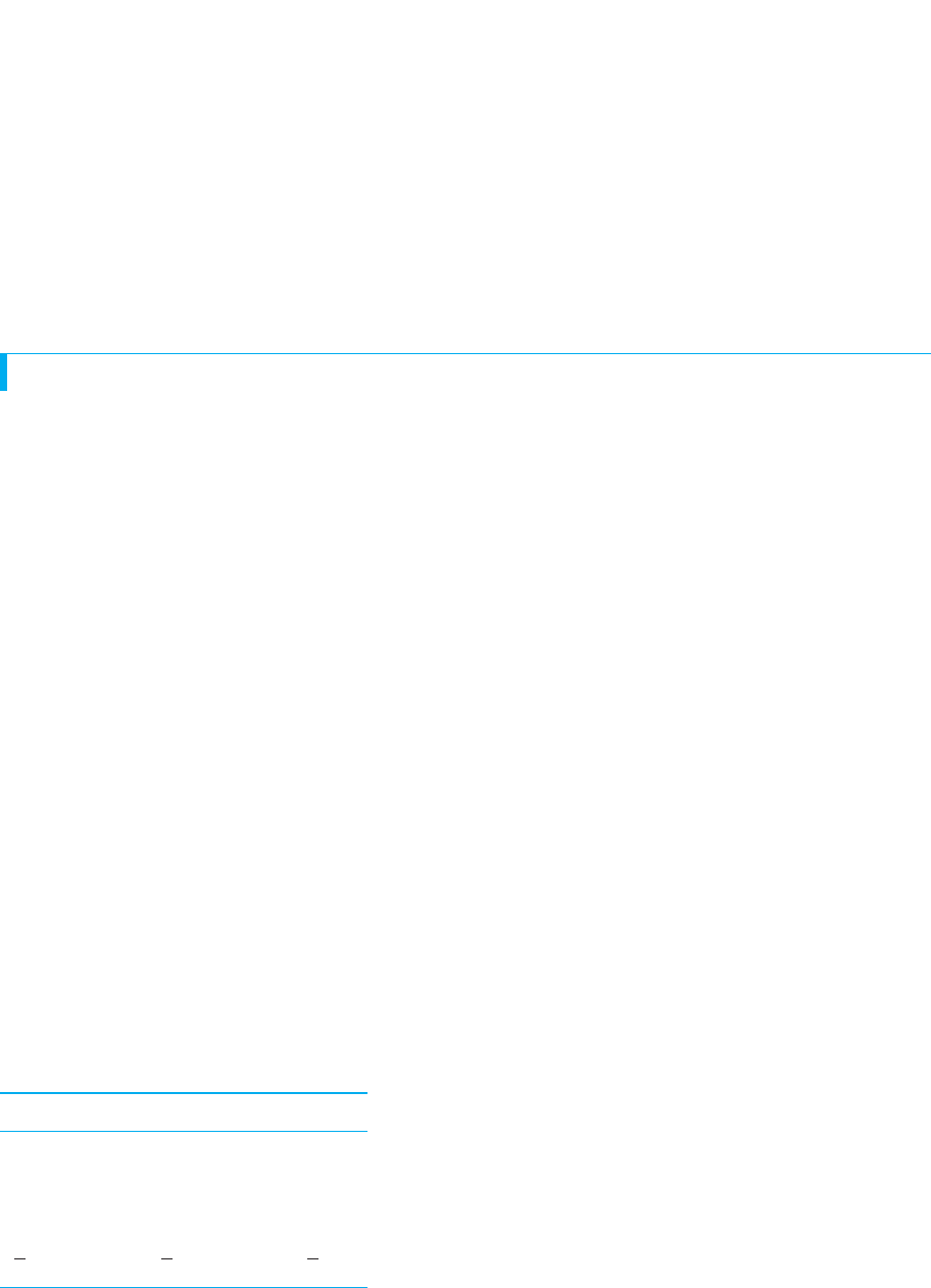
In research publications, we essentially assume that a graph for the population

would be similar to our previous line graph of the sample data. However, so that you

can understand some statistical concepts we will discuss later, you should envision the

relationship in the population in the following way. Each sample mean provides a

good estimate of the corresponding , indicating approximately where on the depend-

ent variable each population would be located. Further, we’ve assumed that recall er-

rors are normally distributed. Thus, we can envision the relationship in the population

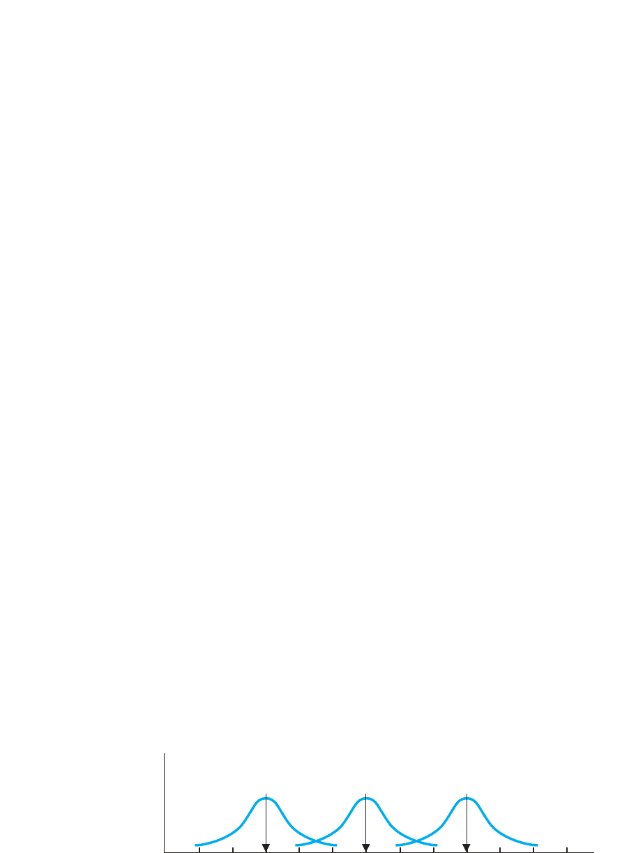
as the normal distributions shown in Figure 4.11. (Note: These are frequency distribu-

tions, so the dependent scores of recall errors are on the axis.) As the conditions of

the independent variable change, scores on the dependent variable increase so that

there is a different, higher population of scores for each condition. Essentially, the dis-

tributions change from one centered around 3 errors, to one around 6 errors, to one

around 9 errors. (The overlap among the distributions simply shows that some people

in one condition make the same number of errors as other people in adjacent condi-

tions.) On the other hand, say that the sample means from our conditions were the

same, such as all equal to 5. Then we would envision the one, same population of

scores, located at the of 5, that we’d expect regardless of our conditions.

Remember that the population of scores reflects the behavior of everyone. If, as the

independent variable changes, everyone’s behavior changes, then we have learned

about a law of nature involving that behavior. Above, we believe that everyone’s recall

behavior tends to change as list length changes, so we have evidence of how human

memory generally works in this situation. That’s about all there is to it; we have basi-

cally achieved the goal of our research.

The process of arriving at the above conclusion sounds easy because it is easy. In

essence, statistical analysis of most experiments involves three steps: (1) Compute each

sample mean (and other descriptive statistics) to summarize the scores and the relation-

ship found in the experiment, (2) Perform the appropriate inferential procedure to de-

termine whether the data are representative, and (3) Determine the location of the

␮

1␮2

FIGURE 4.11

Locations of populations

of error scores as a func-

tion of list length

Each distribution contains

the scores we would expect to

find if the population were

tested under a condition.

0 123456789101112

Recall errors

μ for

5-item

list

μ for

10-item

list

μ for

15-item

list

population of scores that you expect would be found for each condition by estimating

each . Once you’ve described the expected population for each condition, you are ba-

sically finished with the statistical analysis.

REMEMBER Envision a normal distribution located at the for each condi-

tion when envisioning the relationship in the population from an experiment.

STATISTICS IN PUBLISHED RESEARCH: USING THE MEAN

When reading a research article, you may be surprised by how seldom the word rela-

tionship occurs. The phrase you will see instead is “a difference between the means.”

As we saw, when the means from two conditions are different numbers, then each con-

dition is producing a different batch of scores, so a relationship is present. Thus, re-

searchers often communicate that they have found a relationship by saying that they

have found a difference between two or more means. If they have not found a relation-

ship, then they say no difference was found.

One final note: Research journals that follow APA’s publication guidelines do not use

the statistical symbol for the sample mean ( ). Instead, the symbol is . When describ-

ing the population mean, however, is used. (For the median, is used.)Mdn␮

␮

Chapter Summary 79

The mean is the measure of central tendency in behavioral research. You should under-

stand the mode and the median, but the most important topics in this chapter involve

the mean, because they form the basis for virtually everything else that we will discuss.

In particular, remember that the mean is the basis for interpreting most studies. You will

always want to say something like “the participants scored around 3” in a particular

condition because then you are describing their typical behavior in that situation. Thus,

regardless of what other fancy procedures we discuss, remember that to make sense out

of your data you must ultimately return to identifying around where the scores in each

condition are located.

Using the SPSS Appendix: See Appendix B.3 to compute the mean, median, and

mode for one sample of data, along with other descriptive statistics we’ll discuss. For

experiments, we will obtain the mean for each condition as part of performing the

experiment’s inferential procedure.

CHAPTER SUMMARY

1. Measures of central tendency summarize the location of a distribution on a

variable, indicating where the center of the distribution tends to be.

2. The mode is the most frequently occurring score or scores in a distribution. It is

used primarily to summarize nominal data.

3. The median, symbolized by Mdn, is the score at the 50th percentile. It is used

primarily with ordinal data and with skewed interval or ratio data.

4. The mean is the average score located at the mathematical center of a distribution.

It is used with interval or ratio data that form a symmetrical, unimodal distri-

bution, such as the normal distribution. The symbol for a sample mean is , and

the symbol for a population mean is .␮

PUTTING IT

ALL TOGETHER

80 CHAPTER 4 / Measures of Central Tendency: The Mean, Median, and Mode

5. Transforming raw scores by using a constant results in a new value of the mean,

median, or mode that is equal to the one that would be obtained if the transforma-

tion were performed directly on the old value.

6. The amount a score deviates from the mean is computed as .

7. The sum of the deviations around the mean, , equals zero. This makes

the mean the best score to use when predicting any individual score, because the

total error across all such estimates will equal zero.

8. In graphing the results of an experiment, the independent variable is plotted on the

axis and the dependent variable on the axis. A line graph is created when the in-

dependent variable is measured using a ratio or an interval scale. A bar graph is cre-

ated when the independent variable is measured using a nominal or an ordinal scale.

9. On a graph, if the summary data points form a line that is not horizontal, then the

individual scores change as a function of changes in the scores, and a relation-

ship is present. If the data points form a horizontal line, then the scores do not

change as a function of changes in the scores, and a relationship is not present.

10. A random sample mean is the best estimate of the corresponding population’s

mean . The in each condition of an experiment is the best estimate of the

that would be found if the population was tested under that condition.

11. We conclude that a relationship in the population is present when we infer

different values of , implying different distributions of dependent scores, for two

or more conditions of the independent variable.

␮

␮X

1␮2

1X2

1X 2 X2

Mdn

bar graph 76

bimodal distribution 62

deviation 69

line graph 75

mean 66

␮Σ1X 2 X

2XΣX

measure of central tendency 61

median 63

mode 62

sum of the deviations around the mean 70

sum of 60

unimodal distribution 62

KEY TERMS

REVIEW QUESTIONS

(Answers for odd-numbered problems are in Appendix D.)

1. What does a measure of central tendency indicate?

2. What two aspects of the data determine which measure of central tendency to use?

3. What is the mode, and with what type of data is it most appropriate?

4. What is the median, and with what type of data is it most appropriate?

5. What is the mean, and with what type of data is it most appropriate?

6. Why is it best to use the mean with a normal distribution?

7. Why is it inappropriate to use the mean with a skewed distribution?

8. Which measure of central tendency is used most often in behavioral research? Why?

9. What two pieces of information about the location of a score does a deviation

score convey?

10. Why do we use the mean of a sample to predict any score that might be found in

that sample?

11. (a) What is the symbol for a score’s deviation from the mean? (b) What is the

symbol for the sum of the deviations? (c) What does it mean to say “the sum of

the deviations around the mean equals zero”?

12. What is and how do we usually determine its value?

APPLICATION QUESTIONS

13. For the following data, compute (a) the mean and (b) the mode.

55 57 59 58 60 57 56 58 61 58 59

14. (a) In question 13, what is your best estimate of the median (without computing

it)? (b) Explain why you think your answer is correct. (c) Calculate the

approximate median using the method described in this chapter.

15. A researcher collected the following sets of data. For each, indicate the measure of

central tendency she should compute: (a) the following IQ scores: 60, 72, 63, 83,

68, 74, 90, 86, 74, and 80; (b) the following error scores: 10, 15, 18, 15, 14, 13, 42,

15, 12, 14, and 42; (c) the following blood types: O,

O, O, and (d) the following grades: B, D, C, A, B, F, C, B, C, D, and D.

16. You misplaced two of the scores in a sample, but you have the data indicated be-

low. What should you guess the missing scores to be? Why?

7121314111413131211

17. On a normal distribution of scores, four participants obtained the following

deviation scores: , 0, and (a) Which person obtained the lowest raw

score? How do you know? (b) Which person’s raw score had the lowest

frequency? How do you know? (c) Which person’s raw score had the highest

frequency? How do you know? (d) Which person obtained the highest raw

score? How do you know?

18. In a normal distribution of scores, five participants obtained the following devi-

ation scores: , and . (a) Which score reflects the highest raw

score? (b) Which score reflects the lowest raw score? (c) Rank-order the devia-

tion scores in terms of their frequency, starting with the score with the lowest

frequency.

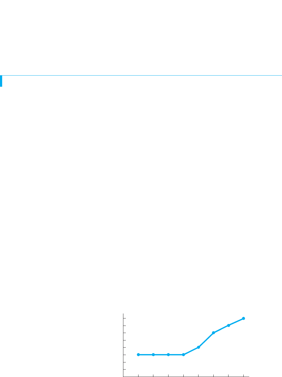
19. For the following experimental results, interpret specifically the relationship

between the independent and dependent variables:

21015,2211,

11.13,25

AB1;

A2, A2, O, A1, AB2, A1,

␮

Application Questions 81

156

Hours of sleep deprivation

24 78

Mean number of errors

82 CHAPTER 4 / Measures of Central Tendency: The Mean, Median, and Mode

20. (a) In question 19, give a title to the graph, using “as a function of.” (b) If you par-

ticipated in the study in question 19 and had been deprived of 5 hours of sleep,

how many errors do you think you would make? (c) If we tested all people in the

world after 5 hours of sleep deprivation, how many errors do you think each

would make? (d) What symbol stands for your prediction in part c?

21. Foofy says a deviation of is always better than a deviation of . Why is she

correct or incorrect?

22. You hear that a line graph of data from the Grumpy Emotionality Test slants

downward as a function of increases in the amount of sunlight present on the day

participants were tested. (a) What does this tell you about the mean scores for the

conditions? (b) What does this tell you about the raw scores for each condition?

(d) What do you conclude about whether there is a relationship between

emotionality and sunlight in nature?

23. You conduct a study to determine the impact that varying the amount of noise

in an office has on worker productivity. You obtain the following productivity

scores.

Condition 1: Condition 2: Condition 3:

Low Noise Medium Noise Loud Noise

15 13 12

19 11 9

13 14 7

13 10 8

(a) Assuming that productivity scores are normally distributed ratio scores, com-

pute the summaries of this experiment. (b) Draw the appropriate graph for these

data. (c) Assuming that the data are representative, draw how we would envision

the populations produced by this experiment. (d) What conclusions should you

draw from this experiment?

24. Assume that the data in question 25 reflect a highly skewed interval variable. (a)

Compute the summaries of these scores. (b) What conclusion would you draw

from the sample data? (c) What conclusion would you draw about the populations

produced by this experiment?

INTEGRATION QUESTIONS

25. (a) How do you recognize the independent variable of an experiment? (b) How do

you recognize the dependent variable? (Ch. 2)

26. (a) What is the rule for when to make a bar graph in any type of study? (b)

Variables using what scales meet this rule? (c) How do you recognize such scales?

(d) What is the rule for when to connect data points with lines? (e) Variables using

what scales meet this rule? (f) How do you recognize such scales? (Chs. 2, 3)

27. When graphing the results of an experiment: (a) Which variable is plotted on the

axis? (b) Which variable is plotted on the axis. (c) When do you produce a bar

graph or a line graph? (Chs. 3, 4)

␮

2515

28. Foofy conducts an experiment in which participants are given 1, 2, 3, 4, 5, or 6

hours of training on a new computer statistics program. They are then tested on

the speed with which they can complete several analyses. She summarizes her

results by computing that the mean number of training hours per participant is 3.5,

and so she expects would also be 3.5. Is she correct? If not, what should she do?

(Chs. 2, 4)

29. For each of the experiments below, determine (1) which variable should be plotted

on the Y axis and which on the X axis, (2) whether the researcher should use a

line graph or a bar graph to present the data, and (3) how she should summarize

scores on the dependent variable: (a) a study of income as a function of age; (b) a

study of politicians’ positive votes on environmental issues as a function of the

presence or absence of a wildlife refuge in their political district; (c) a study of

running speed as a function of carbohydrates consumed; (d) a study of rates of

alcohol abuse as a function of ethnic group. (Chs. 2, 4)

30. Using independent and dependent: In an experiment, the characteristics of the

___________ variable determine the measure of central tendency to compute,

and the characteristics of the ___________ variable determine the type of graph

to produce. (Chs. 2, 4)

■ ■ ■ SUMMARY OF

FORMULAS

␮

Integration Questions 83

1. The formula for the sample mean is

2. The formula for a score’s deviation is X 2 X

X 5

ΣX

3. To estimate the median, arrange the scores in

rank order. If is an odd number, the score in

the middle position is roughly the median. If is

an even number, the average of the two scores in

the middle positions is roughly the median.

So far you’ve learned that applying descriptive statistics involves considering the shape

of the frequency distribution formed by the scores and then computing the appropriate

measure of central tendency. This information simplifies the distribution and allows

you to envision its general properties.

But not everyone will behave in the same way, and so there may be many, very dif-

ferent scores. Therefore, to have a complete description of any set of data, you must

also answer the question “Are there large differences or small differences among the

scores?” This chapter discusses the statistics for describing the differences among

scores, which are called measures of variability. The following sections discuss (1) the

concept of variability, (2) how to compute statistics that describe variability, and

(3) how to use these statistics in research.

First, though, here are a few new symbols and terms.

NEW STATISTICAL NOTATION

A new symbol you’ll see is , which indicates to find the sum of the squared :

First square each and then find the sum of the squared . Thus, to find for the

scores 2, 2, and 3, we have , which becomes , which equals 17.

We have a similar looking operation called the squared sum of that is symbolized

by . Work inside the parentheses first, so first find the sum of the scores and

then square that sum. Thus, to find for the scores 2, 2, and 3, we have

, which is , which is 49. Notice that for the same scores of 2, 2, and

3, produced 17, while produced the different answer of 49. Be careful when

dealing with these terms.

1ΣX2

ΣX

172

12 1 2 1 32

1ΣX2

X1ΣX

4 1 4 1 92

1 2

1 3

ΣX

XsX

XsΣX

Measures of Variability:

Range, Variance, and

Standard Deviation

GETTING STARTED

To understand this chapter, recall the following:

■

From Chapter 4, what the mean is, what and stand for, and what

deviations are.

Your goals in this chapter are to learn

■

What is meant by variability.

■

What the range indicates.

■

When the standard deviation and variance are used and how to interpret them.

■

How to compute the standard deviation and variance when describing a sample,

when describing the population, and when estimating the population.

■

How variance is used to measure errors in prediction and what is meant by

accounting for variance.

X

REMEMBER indicates the sum of squared Xs, and indicates the

squared sum of X.

With this chapter we begin using subscripts. Pay attention to subscripts because they

are part of the symbols for certain statistics.

Finally, some statistics will have two different formulas, a definitional formula and a

computational formula. A definitional formula defines a statistic and helps you to un-

derstand it. Computational formulas are the formulas to use when actually computing a

statistic. Trust me, computational formulas give exactly the same answers as defini-

tional formulas, but they are much easier and faster to use.

WHY IS IT IMPORTANT TO KNOW ABOUT MEASURES OF VARIABILITY?

Computing a measure of variability is important because without it a measure of cen-

tral tendency provides an incomplete description of a distribution. The mean, for exam-

ple, only indicates the central score and where the most frequent scores are. You can

see what’s missing by looking at the three samples in Table 5.1. Each has a mean of 6,

so if you didn’t look at the distributions, you might think that they are identical. How-

ever, sample A contains scores that differ greatly from each other and from the mean.

Sample B contains scores that differ less from each other and from the mean. In sample

C no differences occur among the scores.

Thus, to completely describe a set of data, we need to know not only the central ten-

dency but also how much the individual scores differ from each other and from the cen-

ter. We obtain this information by calculating statistics called measures of variability.

Measures of variability describe the extent to which scores in a distribution differ

from each other. With many, large differences among the scores, our statistic will be a

larger number, and we say the data are more variable or show greater variability.

Measures of variability communicate three related aspects of the data. First, the

opposite of variability is consistency. Small variability indicates few and/or small

differences among the scores, so the scores must be consistently close to each other

(and reflect that similar behaviors are occurring). Conversely, larger variability indi-

cates that scores (and behaviors) were inconsistent. Second, recall that a score indicates

a location on a variable and that the difference between two scores is the distance that

separates them. From this perspective, by measuring differences, measures of variabil-

ity indicate how spread out the scores and the distribution are. Third, a measure of vari-

ability tells us how accurately the measure of central tendency describes the

distribution. Our focus will be on the mean, so the greater the variability, the more the

scores are spread out, and the less accurately they are summarized

by the one, mean score. Conversely, the smaller the variability, the

closer the scores are to each other and to the mean.

Thus, by knowing the variability in the samples in Table 5.1,

we’ll know that sample C contains consistent scores (and behav-

iors) that are close to each other, so 6 accurately represents them.

Sample B contains scores that differ more—are more spread out—

so they are less consistent, and so 6 is not so accurate a summary.

Sample A contains very inconsistent scores that are spread out far

from each other, so 6 does not describe most of them.

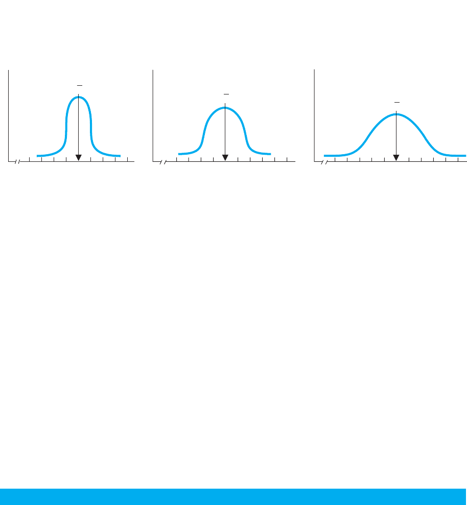
You can see the same aspects of variability with larger distribu-

tions. For example, consider the three distributions in Figure 5.1

1ΣX2

ΣX

Why is it Important to Know About Measures of Variability? 85

TABLE 5.1

Three Different Distributions

Having the Same Mean Score

Sample A Sample B Sample C

086

276

666

10 5 6

12 4 6

X 5 6X 5 6X 5 6

86 CHAPTER 5 / Measures of Variability: Range, Variance, and Standard Deviation

A QUICK REVIEW

■

Measures of variability describe the amount that

scores differ from each other.

■

When scores are variable, we see frequent and/or

large differences among the scores, indicating that

participants are behaving inconsistently.

MORE EXAMPLES

If a survey produced high variability, then each person

had a rather different answer—and score—than the

next. This produces a wide normal curve. If the variabil-

ity on an exam is small, then many students obtained

either the same or close to the same score. This produces

a narrow normal curve.

For Practice

1. When researchers measure the differences among

scores, they measure ____.

2. The opposite of variability is ____.

continued

using our a “parking lot approach.” If our statistics indicate very small variability, we

should envision a polygon similar to Distribution A: It is narrow or “skinny” because

most people in the parking lot are standing in line at their scores close to the mean

(with few at, say, 45 and 55). We envision such a distribution, because it produces

small differences among the scores, and thus will produce a measure of variability

that is small. However, a relatively larger measure of variability indicates a polygon

similar to Distribution B: It is more spread out and wider, because longer lines of

people are at scores farther above and below the mean (more people scored near 45

and 55). This will produce more frequent and/or larger differences among the scores

and this produces a measure of variability that is larger. Finally, very large variability

suggests a distribution similar to Distribution C: It is very wide because people

are standing in long lines at scores that are farther into the tails (scores near 45 and

55 occur very often). Therefore, frequently scores are anywhere between very low

and very high, producing many large differences, which produce a large measure of

variability.

REMEMBER Measures of variability communicate the differences among the

scores, how consistently close to the mean the scores are, and how spread out

the distribution is.

FIGURE 5.1

Three variations of the normal curve

Scores

Distribution A

Distribution B

Scores

Distribution C

30 35 40 45 50 55 60 65 70 0 30 35 40 45 50 55 60 65 70 75

0 3035404550556065707525

For example, the scores of 0, 2, 6, 10, 12 have a range of 12 0 12. The less vari-

able scores of 4, 5, 6, 7, 8 have a range of 8 4 4. The perfectly consistent sample

of 6, 6, 6, 6, 6 has a range of 6 6 0.

Thus, the range does communicate the spread in the data. However, the range is a

rather crude measure. It involves only the two most extreme scores it is based on the

least typical and often least frequent scores. Therefore, we usually use the range as our

sole measure of variability only with nominal or ordinal data.

With nominal data we compute the range by counting the number of categories we

have. For example, say we ask participants their political party affiliation: We have

greater consistency if only 4 parties are mentioned than if 14 parties are reported. With

ordinal data the range is the distance between the lowest and highest rank: If 100 run-

ners finish a race spanning only the positions from first through fifth, this is a close race

with many ties; if they span 75 positions, the runners are more spread out.

It is also informative to report the range along with the following statistics that are

used with interval and ratio scores.

UNDERSTANDING THE VARIANCE AND STANDARD DEVIATION

Most behavioral research involves interval or ratio scores that form a normal distribu-

tion. In such situations (when the mean is appropriate), we use two similar measures of

variability, called the variance and the standard deviation.

Understand that we use the variance and the standard deviation to describe how dif-

ferent the scores are from each other. We calculate them, however, by measuring how

much the scores differ from the mean. Because the mean is the center of a distribution,

when scores are spread out from each other, they are also spread out from the mean.

When scores are close to each other, they are also close to the mean.

This brings us to an important point. The mean is the score around which a distribu-

tion is located. The variance and standard deviation allow us to quantify “around.” For

Understanding the Variance and Standard Deviation 87

The formula for computing the range is

Range  highest score  lowest score

THE RANGE

One way to describe variability is to determine how far the lowest score is from the

highest score. The descriptive statistic that indicates the distance between the two most

extreme scores in a distribution is called the range.

3. When the variability in a sample is large, are the

scores close together or very different from each

other?

4. If a distribution is wide or spread out, then the

variability is ____.

Answers

1. variability

2. consistency

3. different

4. large