Genshiro Kitagawa. Introduction to Time Series Modeling (Введение в моделирование временных рядов)

Подождите немного. Документ загружается.

DECOMPOSITION INCLUDING AN AR COMPONENT 179

12.3 Decomposition Including a Stationary AR Component

In this section, we consider an extension of the standard seasonal adjust-

ment method (Kitagawa and Gersch (1984)). In the standard seasonal

adjustment method, the time series is decomposed into three compo-

nents, i.e., the trend component, the seasonal component and the ob-

servation no ise. These components are assumed to follow the models

given in (12.15) and (12.16), and the observation noise is assumed to

be a white noise. Therefore, if a signiﬁcant deviation from that assump-

tion is present, th e n the decomposition obtained by the standard seasonal

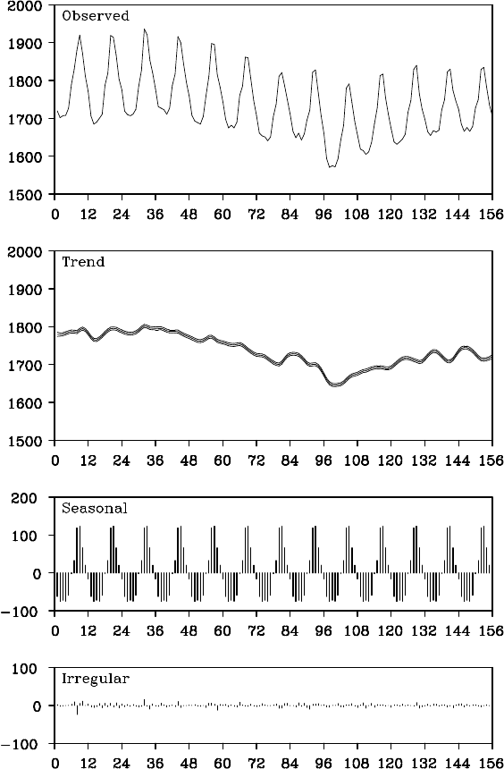
adjustment method might become inappropriate. Figure 12.3 shows the

decomp osition of the BLSALLFOOD data of Figure 1.1(d) that was ob-

tained by the seasonal adjustment method for the model with k = 2, ℓ = 1

and p = 12. In this case, different f rom th e case shown in the previous

section, the estimated trend shows a wiggle, par ticularly in the latter par t

of the data.

Let us consider the problems when the above-men tioned wiggly

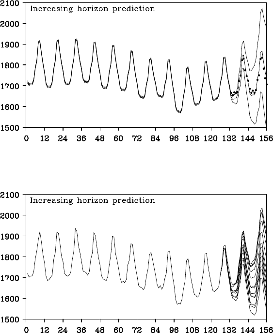
trend is obtaine d. Similarly to the Figure 12.2, Figure 12.4 shows the

increasing hor iz on prediction for the latter two years (24 observations)

of the BLSALLFOOD data based on the fo rmer 132 observations. In

this case, apparently the predicted mean y

132+ j|132

provides a reason able

prediction of the actual time series y

132+ j

. However, it is evident that

prediction by this model is not reliable , because an explosive increase in

the size of the conﬁdence interval is observed.

Figure 12.5 shows the overlay o f 13 increa sin g h orizon predictions

that are obtaine d by assuming the starting point to be n = 126,...,138,

respectively. The increasing hor iz on predictions starting at and before

n = 130 have signiﬁcan t downward bias. On the other hand, the increas-

ing horizon predictions starting at and after n = 135 have signiﬁcant up-

ward bias. This is the reason that the explosive increase in the width of

the conﬁde nce interval of the increasing horizon p redictions has occurred

as the lead time has increased. The stochastic trend component model

in the seasonal adjustment model can ﬂexibly express a complex trend

component. But in the incre asing horizon prediction with this model, th e

predicted mean t

n+ j|n

can simply be obtained b y using the difference

equation

∆

n+ j|n

= 0. (12.21)

Therefore, whether the predicted values may go up or down is de-

cided by the starting point o f the trend. From these results, we see that

if the estimated trend is wiggly, it is not appropriate to use the standard

180 THE SEASONAL ADJUSTMENT MODEL

Figure 12.3 Seasonal adjustment of BLSALLFOOD data by the standard sea-

sonal adjustment model.

DECOMPOSITION INCLUDING AN AR COMPONENT 181

Figure 12.4 Increasing horizon prediction of BLSALLFOOD data (prediction

starting point: n = 132).

Figure 12.5 Increasing horizon prediction of BLSALL FOOD data with ﬂoating

starting points (prediction starting point: n =126, . . . , 138).

seasonal adjustment mode l for increasing horizon prediction.

In predicting one year or two years ahead, it is possible to obtain a

better prediction with a smooth er curve by using a smaller value than the

maximum likelihood estimate for the system noise variance of the trend

component,

. However, this method suffers from the following p rob-

lems; it is difﬁcult to reasonably determine

and, moreover, prediction

182 THE SEASONAL ADJUSTMENT MODEL

with a small lead time such as one-step- ahead prediction becomes sig-

niﬁcantly worse than that obtained by the ma ximum likelihood model.

To achieve good prediction for both short and long lead times, we

consider an extension of the standard seasonal adjustment model by in-

cluding a new component p

= t

+ s

+ p

+ w

. (12.22)

Here, p

is a stationary AR component model that is assumed to follow

an AR mode l

∑

i=1

n−i

+ v

, (12.23)

where v

is assum ed to b e a Gaussian white noise with mean 0 and

variance

. This model expresses a short-term variation, for instance,

the cycle of an economic time series, not a long-term tendency like the

trend component. In the model (12.22), the trend component obtained by

the standard seasonal adjustment mo del is further dec omposed into the

smoother trend component t

and the sh ort-term variation p

. As shown

in Chapter 9, the state-space rep resentation of the AR model (12.22) is

obtained by deﬁning the state vector x

= (p

, p

n−1

,.. ., p

n−m

)

and







··· a







, G













, (12.24)

= [

1 0 ··· 0

], Q

Therefore, using the state-space representation for the composite

model shown in Ch a pter 9, the state-space model for the d e composition

of (12.22) is obtained by d eﬁning

F =









, G =





0 0

0 G

0 0 G





H = [

], Q =





0 0





. (12.25)

DECOMPOSITION INCLUDING AN AR COMPONENT 183

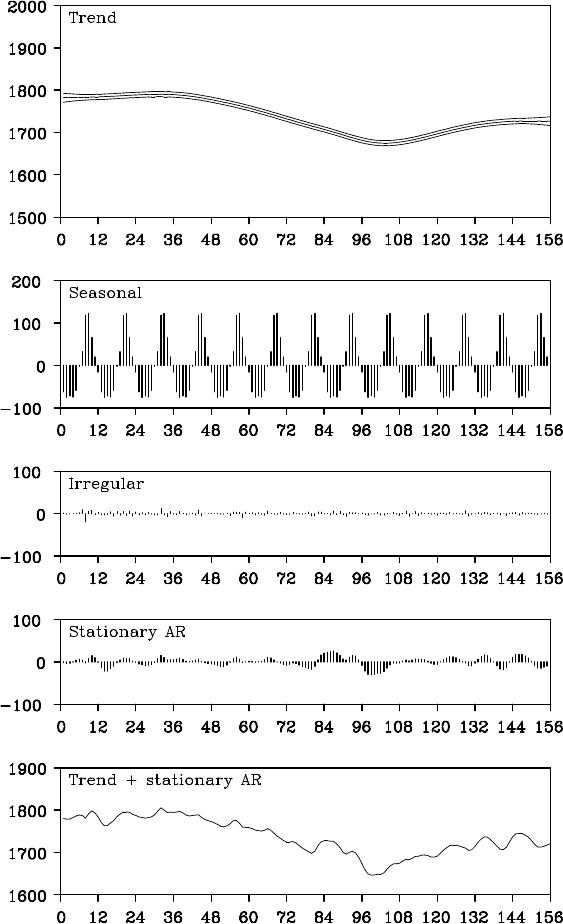
Figure 12.6 Seasonal adjustment of BLSALLFOOD data by the model, including

stationary AR components.

184 THE SEASONAL ADJUSTMENT MODEL

Example (Seasonal adjustment with stationary AR component)

Figure 12.6 shows the decomposition of BLSALLFOOD data into

trend, seasonal, stationary AR and obser vation no ise components by th is

model. The estimated trend expresses a very smooth c urve similar to

Figure 12.1. On the other ha nd, a short-term variation is detected as

the stationary AR component and the (trend component) + (stationary

AR component) resemble the trend compon e nt of Figure 12.3. The AIC

value for this model is 1336.54, which is signiﬁcantly smaller than that

of the standard seasonal adjustment model, 1369.30.

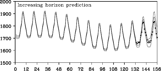
Figure 12. 7 shows the increasing horizon pred iction with this model

starting from n = 132. It can be seen that a good prediction was ac hieved

with both short and long lead time s.

Figure 12.7 Increasing horizon prediction of the BLSALLFOOD data by the

model, including stationary AR components.

12.4 Decomposition Including a Trading-Day Effect

Monthly economic time ser ies, such as the amount of sales at a depart-

ment store, may strongly depend on the numbe r of the days of the week

in each month, because there are m arked differences in sales depending

on the days of the week. For example, a department store may have m ore

customers on Saturdays and Sunday s or may r egu la rly close on a speciﬁc

day of a week. A similar phenomenon can often be seen in environmental

data, for example, the daily amounts of NO

and CO

recorde d.

A trading-day adjustment has b een developed to remove such

trading- day effects tha t depend on the number of the day s of the

week (Cleveland and Devlin (1980), Hillmer (1982)). To develop a

DECOMPOSITION INCLUDING A TRADING-DAY EFFECT 1 85

model-based method for trading-day adjustme nt, we have to develop a

proper model for the trading-day effect component (Akaike and Ishiguro

(1983), K itagawa and Gersch (1984, 1996)). Hereinafter, the numbers

from Sunday to Saturday in the n-th data, y

, are denoted as d

∗

,···, d

∗

Note that each d

∗

takes a value 4 or 5 for monthly d ata. Then the

effect of the trading-day is expressed as

∑

i=1

∗

. (12.26 )

The coefﬁcient

expresses the effect of the number of the i-th day

of the week on the value of y

. Here, to guarantee unique ness of the

decomp osition of the time series, we impose the restriction on it that the

sum of all coefﬁcients amounts to 0, that is,

+ ···+

= 0. (12.27)

Since the last coefﬁcient is deﬁned by

= −(

+ ···+

), the

trading- day effect can be expressed by using

,.. .,

∑

i=1

∗

−d

∗

)

≡

∑

i=1

, (12.28)

where d

≡ d

∗

−d

∗

is the difference in the number of the i- th day of

the week and th e numb er of Saturdays in the n-th month c orrespond ing

to y

On the a ssumption that these coefﬁcients gradually change, follow-

ing the ﬁrst order trend m odel

∆

= v

(i)

, v

(i)

∼ N(0,

), i = 1,. .., 6, (12.29)

the state-space representation of the trading-d a y effect model is obtained

= G

= I

, H

= [d

,.. ., d

]













, Q =













. (12.30)

186 THE SEASONAL ADJUSTMENT MODEL

In this representation, H

becomes a time-dependent vector. For sim-

plicity, the variance-covariance matrix Q is assumed to be a diagonal

matrix with equal diagonal elements. In actual analysis, however, we of-

ten assume that the coefﬁcients are time-invariant, i.e.,

≡

, (12.31)

where we may put either

= 0 or G = 0 for the state-space representa-

tion of this mode l.

The state-space model for the decomposition of the time series

= t

+ s

+ p

+ td

+ w

(12.32)

can be obtain e d by using













, F =













, G =







0 0

0 G

0 0 G

0 0 0







H = [

], Q =





0 0





. (12.33)

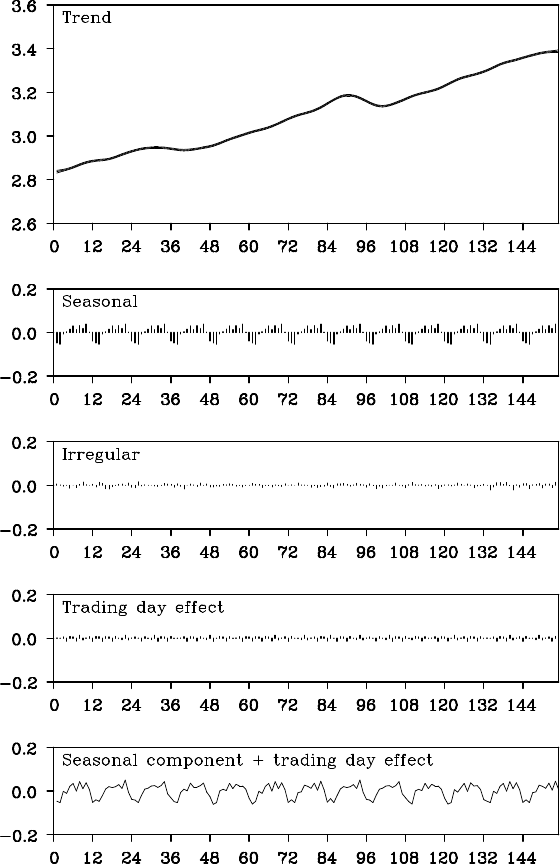
Example (Seasonal adjustment with trading-day effect) Figure

12.8 shows th e results of the logarithm of the WHARD data, the de-

composition into the trend, the seasonal, the trading-day effect and the

noise components by the seasonal adjustme nt model with trading- day

effect. The estimated trend and seasonal components are similar to th e

decomp osition by the standard seasonal adjustment model shown in Fig-

ure 1 2.1. Although the extracted trading-day effect component is appar-

ently minuscule, it can be seen that the plot of seasonal co mponent plus

trading- day effect component reproduces the details of the observed time

series. The AIC value for this m odel is −778.18, which is sign iﬁcantly

smaller than that for the standard seasonal adjustment model, −728.50.

Once the time-invariant coefﬁcients of trading-day effects

are esti-

mated, this can contribute to a signiﬁcant increase in the accur acy of

prediction, because d

,···, d

are known, even for the future.

DECOMPOSITION INCLUDING A TRADING-DAY EFFECT 1 87

Figure 12.8: Trading-day adjustment for WHARD data.

188 THE SEASONAL ADJUSTMENT MODEL

Problems

1. D escribe what we should check wh en decomposing a time series us-

ing a seasonal adjustment model with a stationary AR component.

2. Co nsider a different seasonal component model from that given in

12.1.

3. In trading day adjustments, consider a model that takes into account

the following c omponents:

(1) The effects of the wee kend (Saturday and Sunday) and weekdays

are different.

(2) There are th ree different e ffects, i.e., Saturday, Sunday an d the

weekdays.

4. Co nsider any other possible effects related to seasonal adjustments

that are not considered in this book.

5. Try seasonal adjustme nt of an actual time series. You may use the

WebDecomp software at website http://www.ism.ac.jp/˜sato.