Genshiro Kitagawa. Introduction to Time Series Modeling (Введение в моделирование временных рядов)

Подождите немного. Документ загружается.

TREND MODEL 169

the variance ratio of the system noise and th e observation noise. Here

is called a trade-o ff parameter. The order of the tre nd model k can be

determined by the information criterion AIC. O ften for analysis, k = 2 is

used. However, for situations wher e the tren d is variable, k = 1 may be

used instead.

Table 11.3: AIC values for trend models.

k = 1 k = 2

AIC

0.223 ×10

−2

2690 0.321 ×10

−5

2556

0.223 2448 0.321 ×10

−3

2506

0.223 ×10

2528

0.0321 2562

Table 11. 3 summarizes the values of

and AI C for the models used

for Figure 11.2. AIC is minimized at

= 0.223 for k = 1 and at

0.321 ×10

−3

for k = 2. Incidentally, these estimates a re obtained by the

maximum likelihoo d me thod. Comparison of the AIC values for k = 1

and k = 2 reveals that the AIC for k = 1 is signiﬁcantly smaller. It should

be noted that according to the AIC, the wiggly trend obtained using k = 1

is p referable to the nicely smooth trend obtained with k = 2. This is

probably because the no ise w

is assumed to be a white noise; thus, the

trend model is inappropriate for the maximum temperature data.

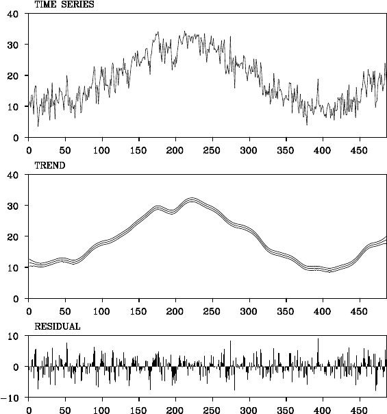
Figure 11.4 shows the observations, the estimated trend and the

residuals when the time series is decomposed by the model, k = 2 and

= 0.321×10

−3

. Obviously, the residuals reveal stron g cor relation an d

does not seem to be a w hite noise sequence.

As shown in the next chapter, we can obtain a smoother trend that ﬁts

the d a ta better using a seasonal adjustment model by decomposing the

time series into three components; tren d, AR component and obser vation

noise. Using a seasonal ad justment model, we can obtain a smoother

trend that better ﬁts the data.

170 ESTIMATION OF TRENDS

Figure 11.4 Temperature data and the trend and residuals obtained by the trend

model with k = 2 and

= 0.321 ×10

−3

Problems

1. According to the rando m walk hypothesis for stock prices, a stock

price y

follows a random walk model y

= y

n−1

+ v

, v

∼N(0,

(1) Assume that y

= 17, 000 and

= 40,000 on a certain day. Obtain

the k-days ahead prediction of the stock price and its pred iction

error variance for k = 1,..., 5.

(2) Obtain the probability that the stock price exceeds 17 ,000 Yen after

4 days have passed.

(3) Do actual stock prices satisfy the rando m walk hypothesis? If not,

consider a modiﬁcation of the model.

TREND MODEL 171

(4) Estimate the trend of actual stock price da ta (N ikkei 225 Japanese

stock price data and software for estimating the trend is given at

the web site http://www.ism.ac.jp/˜sato.)

2. G ive an example of a p arametric trend model other than the polyno-

mial trend model.

Chapter 12

The Seasonal Adjustment Model

The seasona l adjustment model is treated in this cha pter as an example

of extensions of the trend model. Many economic time series repeat-

edly show similar patterns in the vicinity of the same season of every

year. In judging a tenden cy or prediction of such time series, we should

carefully take into account these characteristics to avoid misleading re-

sults. A seasonal adjustment method is developed for analy zing time se-

ries th at repeat similar patterns of variation at constant intervals (Shiskin

(1976), Ak aike (1980ab), Cleveland et al. (1982), Kitagawa and Gersch

(1984)). Seasonal adjustment models decompose a time series y

into

three components of trend t

, seasonal component s

and white noise w

to represent it as y

= t

+ s

+ w

12.1 Seasonal Component Model

In time series, a patterned variation s

that appears rep eatedly every year

is called a seasonal component. In the following, p denotes the pe riod

length of the seasonal c omponen t. Here, we put p = 12 for monthly data

and p = 4 for quarterly data, respectively. Then, the seasonal compon ent

approximately satisﬁes

= s

n−p

. (12.1)

Using the lag operator B, since s

n−p

is denoted as B

, th e seasonal

component approximate ly satisﬁes

(1 −B

= 0. (12.2)

Similar to the stocha stic trend component model introduced in Chap-

ter 11, a model for the seasonal component that g radually changes with

time, is given by (Kitag awa a nd Gersch (1984, 1996))

(1 −B

)

ℓ

= v

, v

∼ N(0,

). (12.3)

In particular, setting ℓ = 1, we ca n obtain a rand om walk model for the

173

174 THE SEASONAL ADJUSTMENT MODEL

seasonal component by

= s

n−p

+ v

. (12.4 )

In this model, it is assumed that s

pn+i

, n = 1,2, ... is a random walk for

any i = 1, ... , p.

Therefore, assuming that the time series consists of the trend compo-

nent t

, the seasonal component s

and the obser vation noise w

, we can

obtain a basic model for seasonal adjustment as

= t

+ s

+ w

, (12.5)

with the trend component model (11 .15) in the previous chapter and th e

above seasonal component model (12.3).

However, the apparently most natural model (12.4) fo r seasonal ad-

justment may not work well in practice, beca use the trend component

model and the seaso nal component model both con ta in the common fac-

tor (1 −B)

, (q ≥ 1). This can be seen by comparing the back-shift op-

erator expression of the trend model (11.18) to the seasonal component

model (12.3 ) with the decomposition

(1 −B

)

ℓ

= (1 −B)

ℓ

(1 + B + ···+ B

p−1

)

ℓ

Here, assume that e

is an arbitrary solution of the difference equation

(1 −B)

= 0. (12.6)

For q = 1, e

is an arbitra ry constant. If we deﬁne new components t

′

and s

′

= t

+ e

′

= s

−e

then they satisfy (11.15), (12.3) and

= t

′

+ s

′

+ w

. (12.7)

Therefore, we have inﬁnitely ma ny ways to decompose the time series

yielding the same noise inputs v

, v

and w

. Moreover, since the likeli-

hood of the model corresponding to those deco mpositions is determined

only by v

, v

and w

, it is impossible to discriminate between the

goodness of the decompositions by the likelihood. Once we use compo-

nent models with common factors, we lose uniqueness of the decompo-

sition.

SEASONAL COMPONENT MODEL 175

A simple method to guar antee uniqueness of deco mposition is to

ensure that none of the component models share any com mon factors.

Since 1 −B

= (1 −B)(1 + B + ···+ B

p−1

) and the sufﬁcient condition

for (1 −B

)

ℓ

= 0 is

(1 + B + ···+ B

p−1

)

ℓ

= 0, (12.8)

≈ S

n−p

is attained, if

p−1

∑

i=0

≈ 0 (12.9)

is satisﬁed. Therefore, as a stoc hastic model of a seasonal compon ent

that gradually changes with time, we may use the following model:



p−1

∑

i=0



ℓ

= v

, v

∼ N





. (12.10)

In this book, the above model is called a seasonal compone nt mod el

with period p and order ℓ. In actual ana lysis, except for situations where

the seasonal co mponent shows a signiﬁcant trend in its changes, the ﬁrst

order model

p−1

∑

i=0

n−i

= v

, v

∼ N





(12.11)

is usually used.

To obtain a state-space representation of the seasonal component

model, initially we expand the operator in (12.9) as follows:



p−1

∑

i=0



ℓ

= 1 −

ℓ(p−1)

∑

i=1

. (12.12)

The co efﬁcient d

is given by d

= −1,i = 1,..., p −1 fo r ℓ = 1 and d

−i−1, i ≤ p −1, and d

= i +1 −2p, p ≤i ≤2(p−1) for ℓ = 2. Since the

seasonal component model given in (12.12) is formally a sp ecial c a se of

an autoregressive model, the state-space representation of the seasonal

component model can be given as







n−1

n−ℓ(p−1)+1







, F =







··· d

ℓ(p−1)







, G =













H = [ 1, 0, ... , 0 ]. (12.13)

176 THE SEASONAL ADJUSTMENT MODEL

12.2 Standard Seasonal Adjustment Model

For standard seasonal adjustment, the time series y

is decomposed into

the following three components

= t

+ s

+ w

, (12.14)

where t

, s

and w

are the trend component, the seasonal co mponent and

the observation noise, respectively. Combining the basic model (12.12)

with the trend component model and the seasonal component model, we

obtain the following standard seasonal adjustment models,

= t

+ s

+ w

(observation model) (12.15)

△

= v

(trend component model) (1 2.16)



p−1

∑

i=0



ℓ

= v

(seasonal component model)(12.17)

where w

∼ N(0,

), v

∼ N(0,

) and v

∼ N(0,

The above model is called the standard seasonal adjustment mode l.

For a seasonal adjustment model with trend order k, period p and

seasonal order ℓ = 1, le t the (k + p −1) dimensional state vector be

deﬁned by x

= (t

,···,t

n−k+1

n−1

,···, s

n−p+2

)

, and deﬁne a 2-

dimensional noise vector as v

= (v

)

, and the matrices F, G and

H by

F =



O F



, G =



O G



, H = [H

], (12.18)

then the state-space representation of the seasonal adjustment model is

obtained as

= Fx

n−1

+ Gv

= Hx

+ w

. (12 .19)

Here, F

, G

and H

are the matrices and vectors used for the state-

space rep resentation of the trend com ponent model, and similarly, F

and H

are the matrices and vectors used for the representation of the

seasonal component model. For instance, if k = 2, ℓ = 1 and p = 4, then

F, G and H are deﬁned by

F =







2 −1

1 0

−1 −1 −1







, G =







1 0

0 0

0 1

0 0







STANDARD SEASONAL ADJUSTMENT MODEL 177

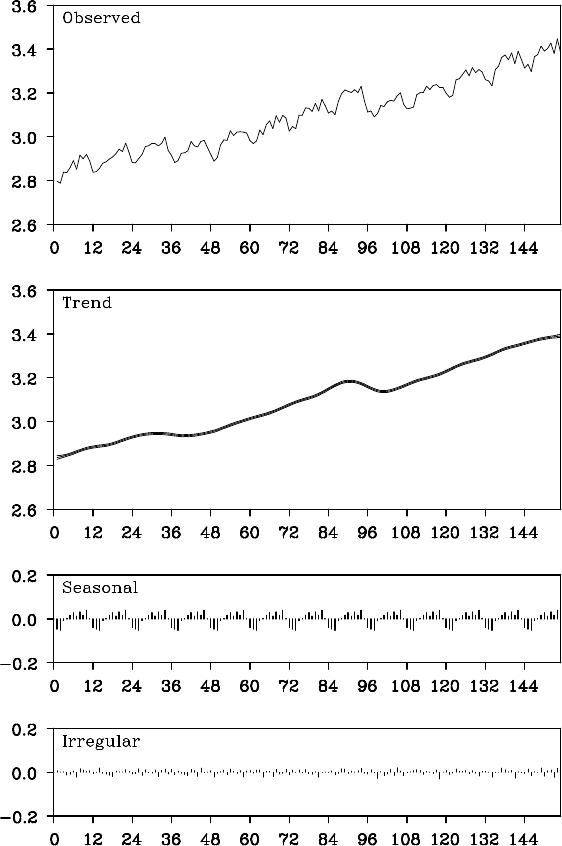
Figure 12.1 Seasonal adjustment of WHARD data by a standard seasonal ad-

justment model.

178 THE SEASONAL ADJUSTMENT MODEL

H = [ 1 0 1 0 0 ]. (12.20)

Example (Seasonal adjustment of WHA RD data) Figure 12 .1

shows the estimates of the trend, the season al and the noise components

of the logarithm of WHARD data using the stan dard seasonal adjust-

ment model. The ma ximum likelihood estimates of the parameters are

= 0.0248,

= 0.11×10

−7

= 0.156×10

−3

, and AIC = −728.50.

Plot (b) in Figure 12.1 shows the estimated trend c omponen t t

n|N

and

±1 standard error interval. A very smooth upward trend is evident, ex-

cept for the years 1974 and 1975 where a rapid decre a se in the trend is

detected, and the estimated seasonal componen t is very stable over the

whole interval.

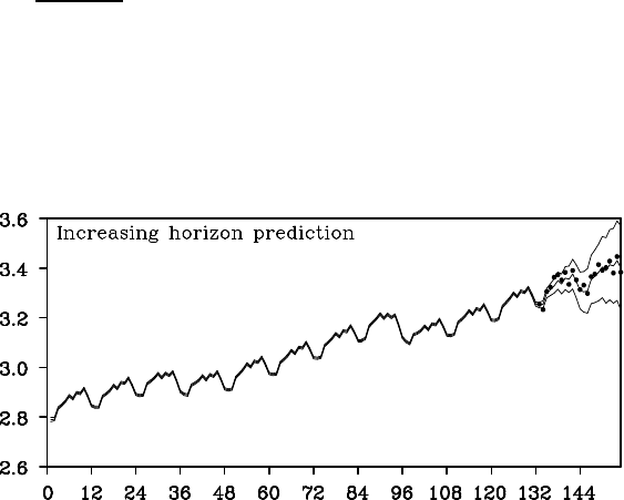
Using the seasonal adjustment model, we can predict time series with

seasonal variation. Figure 12.2 shows the incre asing horizon prediction

over two years, i.e., 24 observations using the initial 132 observations

by the m e thod shown in Chapter 9. In the ﬁgure, the mean of the pre-

dictive distribution y

132+ j|132

and the ±1 standard error interval, i.e.,

132+ j|132

for j = 1,. .., 24 are plotted. The ac tual obser vations are

denoted by the symbol ◦. In this case, very good increasing horizon pre-

diction can be attained, because the estimated trend and seasonal com-

ponen ts are steady. However, it should b e noted tha t ±1 standard error

interval is very wide.

Figure 12.2: Increasing horizon prediction using a seasonal adjustment model.