Gebali F. Analysis Of Computer And Communication Networks
Подождите немного. Документ загружается.

Problems 177
5.9
P =
⎡
⎢
⎢
⎣
10 00.3
00.500
00.510.6
00 00.1
⎤
⎥
⎥
⎦
5.10
P =
⎡
⎢
⎢
⎣
0.70 0 0
0.10.90.20
0.10.10.80
0.10 0 1
⎤
⎥
⎥
⎦
5.11
P =
⎡
⎢
⎢
⎢
⎢
⎣
0.40000
0.20.50.80 0
0.10.50.20 0
0.10 0 0.70.9
0.20 0 0.30.1
⎤
⎥
⎥
⎥
⎥
⎦
5.12
P =
⎡
⎢
⎢
⎢
⎢
⎢
⎢
⎣
0.20 0 0.20 0.6
00.30 0.30 0
000.20.20.30
00.30 0.30 0
00.20.80 0.70
0.80.20000.4
⎤
⎥
⎥
⎥
⎥
⎥
⎥
⎦
Transient Analysis
5.13 Check whether the given transitions matrix is reducible or irreducible. Identify
the closed and transient states and express the matrix in the form of (5.2) or
(5.3) and identify the component matrices C, A, and T.
P =
⎡
⎢
⎢
⎢
⎢
⎣
0.50 00 0.5
00.500.25 0
0010.25 0
00.500.25 0
0.50 00.25 0.5
⎤
⎥
⎥
⎥
⎥
⎦
178 5 Reducible Markov Chains
Find the value of P
10
using (5.8) and (5.9) on page 158 and verify your
results using repeated multiplications.
5.14 Assume the transition matrix P has the structure given in (5.1) or (5.2). Prove
that P
n
also possesses the same structure as the original matrix and prove
also that the component matrices C, A, and T have the same properties as the
original component matrices.
5.15 Find an expression for the transition matrix using (5.13) at time n = 4
and n = 20 for the reducible Markov chain characterized by the transition
matrix
P =
⎡
⎢
⎢
⎢
⎢
⎣
0.70.90.30.30.2
0.30.10.20.10.3
000.20.20
000.20.20.3
000.10.20.2
⎤
⎥
⎥
⎥
⎥
⎦
Find the value of P
10
using (5.8) and verify your results using repeated
multiplications.
Reducible Markov Chains at Steady-State
5.16 In Section 5.7, it was asserted that the transition matrix for a reducible Markov
chain will have the form of (5.22) where all the columns of the matrix are
identical. Prove that assertion knowing that
(a) all the columns of C
1
are all identical
(b) matrix C
1
is column stochastic
(c) matrix Y
∞
is column stochastic
(d) the columns of Y
∞
are identical to the columns of C
1
.
5.17 Find the steady-state transition matrix and distribution vector for the reducible
Markov chain characterized by the matrix
P =
⎡
⎢
⎢
⎢
⎢
⎣
0.90.20.50.10.1
0.10.80.10.20.3
000.20.20.1
000.20.20.1
0000.30.4
⎤
⎥
⎥
⎥
⎥
⎦
Problems 179
5.18 Find the steady-state transition matrix and distribution vector for the reducible
Markov chain characterized by the matrix
P =
⎡
⎢
⎢
⎣
0.90.20.50.1
0.10.80.10.2
000.40.2
0000.5
⎤
⎥
⎥
⎦
5.19 Find the steady-state transition matrix and distribution vector for the reducible
Markov chain characterized by the matrix
P =
⎡
⎢
⎢
⎢
⎢
⎣
0.10.20.50.10.1
0.50.70.10.20.3
0.40.10.40.20.1
0000.20.1
0000.30.4
⎤
⎥
⎥
⎥
⎥
⎦
5.20 Find the steady-state transition matrix and distribution vector for the reducible
Markov chain characterized by the matrix
P =
⎡
⎢
⎢
⎢
⎢
⎣
10.20.20.10.1
00.30.10.20.3
00.10.40.20.1
00.30.10.20.1
00.10.20.30.4
⎤
⎥
⎥
⎥
⎥
⎦
5.21 Find the steady-state transition matrix and distribution vector for the reducible
Markov chain characterized by the matrix
P =
⎡
⎢
⎢
⎢
⎢
⎣
100.20.10.1
010.10.20.3
000.40.20.1
000.10.20.1
000.20.30.4
⎤
⎥
⎥
⎥
⎥
⎦
Note that this matrix has two absorbing states.
5.22 Consider the state transition matrix
P =
⎡
⎣
010
1 − p 0 q
p 01− q
⎤
⎦
180 5 Reducible Markov Chains
(a) Can this matrix represent a reducible Markov chain?
(b) Find the distribution vector at equilibrium.
(c) What values of p and q give s
0
= s
1
= s
2
?
5.23 Consider a discrete-time Markov chain in which the transition probabilities
are given by
p
ij
= q
|i−j|
p
For a 3 × 3 case, what are the values of p and q to make this a reducible
Markov chain? What are the values of p and q to make this an irreducible
Markov chain and find the steady-state distribution vector.
5.24 Consider the coin-tossing Example 5.3 on page 156. Derive the equilibrium
distribution vector and comment on it for the cases p < q, p = q, and p > q.
5.25 Rewrite (5.10) on page 158 to take into account the fact that some of the eigen-
values of C might be repeated using the results of Section 3.14 on page 103.
Identification of Reducible Markov Chains
Use the results of Section 5.9 to verify that the transition matrices in the follow-
ing problems correspond to reducible Markov chains and identify the closed and
transient states. Rearrange each matrix to the standard form as in (5.2) or (5.3).
5.26
P =
⎡
⎣
0.30.10.4
00.10
0.70.80.6
⎤
⎦
5.27
P =
⎡
⎣
0.40.60
0.40.30
0.20.11
⎤
⎦
5.28
P =
⎡
⎢
⎢
⎣
0.50.30 0
0.10.10 0
0.30.40.20.9
0.10.20.80.1
⎤
⎥
⎥
⎦
Problems 181
5.29
P =
⎡
⎢
⎢
⎣
0.10 0 0
0.30.10.50.3
0.40.30.40.2
0.20.60.10.5
⎤
⎥
⎥
⎦
5.30
P =
⎡
⎢
⎢
⎢
⎢
⎣
0.20.30 0.30
0.20.4000
0.30 0.50.10.2
0.20 0 0.40
0.10.30.50.20.8
⎤
⎥
⎥
⎥
⎥
⎦
5.31
P =
⎡
⎢
⎢
⎢
⎢
⎣
0.20.
10.30.10.6
00.30 0.20
0.20.20.40.10.3
00.10 0.40
0.60.30.30.20.1
⎤
⎥
⎥
⎥
⎥
⎦
5.32
P =
⎡
⎢
⎢
⎢
⎢
⎣
0.80.40 0.50
00.1000
00.10.80 0.3
0.20.20 0.50
00.20.20 0.7
⎤
⎥
⎥
⎥
⎥
⎦
5.33
P =
⎡
⎢
⎢
⎢
⎢
⎢
⎢
⎣
0.10 0.
200 0.3
0.20.50.100.40.1
0.10 0.300 0.3
0.20 0.110 0
0.30.50.200.60.1
0.10 0.100 0.2
⎤
⎥
⎥
⎥
⎥
⎥
⎥
⎦
5.34
P =
⎡
⎢
⎢
⎢
⎢
⎢
⎢
⎢
⎢
⎣
0.10.50 0.1000.6
0.70.30 0.2000.3
000.50.30.10 0
0000.20 0.30
000.50 0.90.20
0000.20 0.40
0.
20.20000.10.1
⎤
⎥
⎥
⎥
⎥
⎥
⎥
⎥
⎥
⎦
182 5 Reducible Markov Chains
References
1. R.A. Horn and C.R. Johnson, Matrix Analysis, Cambridge University Press, Cambridge, 1985.

Chapter 6
Periodic Markov Chains
6.1 Introduction
From Chapter 4, we infer that a Markov chain settles down to a steady-state distri-
bution vector s when n →∞. This is true for most transition matrices representing
most Markov chains we studied. However, there are other times when the Markov
chain never settles down to an equilibrium distribution vector, no matter how long
we iterate. So this chapter will illustrate periodic Markov chains whose distribution
vector s(n) repeats its values at regular intervals of time and never settles down to
an equilibrium value no matter how long we iterate.
Periodic Markov chains could be found in systems that show repetitive behavior
or task sequences. An intuitive example of a periodic Markov chain is the population
of wild salmon. In that fish species, we can divide the life cycle as eggs, hatchlings,
subadults, and adults. Once the adults reproduce, they die, and the resulting eggs
hatch and repeat the cycle as shown in Fig. 6.1. Fluctuations in the salmon pop-
ulation can thus be modeled as a periodic Markov chain. It is interesting to note
that other fishes that lay eggs without dying can be modeled as nonperiodic Markov
chains.
Another classic example from nature where periodic Markov chains apply is the
predator–prey relation—where the population of deer, say, is related to the pop-
ulation of wolves. When deer numbers are low, the wolf population is low. This
results in more infant deer survival rate, and the deer population grows during the
next year. When this occurs, the wolves start having more puppies and the wolf
population also increases. However, the large number of wolves results in more
deer kills, and the deer population diminishes. The reduced number of deer results
in wolf starvation, and the number of wolves also decreases. This cycle repeats as
discussed in Problem 6.14.
Another example for periodic Markov chains in communications is data trans-
mission. In such a system, first, data are packetized to be transmitted, and then
the packets are sent over a channel. The received packets are then analyzed for the
presence of errors. Based on the number of bits in error, the receiver is able to correct
for the errors or inform the transmitter to retransmit, perhaps even with a higher level
of data redundancy. Figure 6.2 shows these states which are modeled as a periodic
F. Gebali, Analysis of Computer and Communication Networks,
DOI: 10.1007/978-0-387-74437-7
6,
C
Springer Science+Business Media, LLC 2008
183
184 6 Periodic Markov Chains
Fig. 6.1 Wild salmon can be
modeled as a periodic
Markov chain with the states
representing the number of
each phase of the fish life
cycle
Adults
Eggs
Hatchlings
Subadults
Fig. 6.2 Data communication
over a noisy channel can be
modeled as a periodic
Markov chain with the states
representing the state of each
phase
Transmit
Channel
Reception
Decision
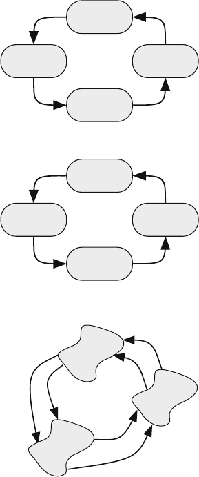
Fig. 6.3 A periodic Markov
chain where states are divided
into groups and allowed
transitions occur only
between adjacent groups
S
2
S
1
S
3
Markov chain. In each transmission phase, there could be several states indicating
the level of decoding required or the number of random errors introduced.
Consider the abstract transition diagram shown in Fig. 6.3, where the states of the
Markov chain are divided into groups and allowed transitions occur only between
adjacent groups. The sets of states S
1
, S
2
, ··· are called periodic classes of the
Markov chain. A state in set S
1
is allowed to make a transition to any other state in
set S
2
only. Thus, the states in the set S
1
cannot make a transition to any state in S
1
or S
3
. A similar argument applies to the states in sets S
2
or S
3
.
6.2 Definition
A periodic Markov chain has the property that the number of single-step transitions
that must be made after leaving a state to return to that state is a multiple of some
6.4 The Transition Matrix 185
integer γ>1 [1]. This definition implies that the distribution vector never settles
down to a fixed steady-state value no matter how long we iterate.
Having mentioned that Markov chains could be periodic, we naturally want to
know how to recognize that the transition matrix P represents a periodic Markov
chain. In addition, we will also want to know the period of such a system. The
theorems presented here will specify the properties of the transition matrix when
the Markov chain is periodic.
Of course, a Markov chain that is not periodic would be called nonperiodic. A
nonperiodic Markov chain does not show repetitive behavior as time progresses,
and its distribution vector settles down to a fixed steady-state value.
6.3 Types of Periodic Markov Chains
There are two types of periodic Markov chains
1. Strongly periodic Markov chains the distribution vector repeats its values with a
period γ>1. In the next section, we will find out that the state transition matrix
satisfies the relation
P
γ
= I. (6.1)
In other words, in a strongly periodic Markov chain, the probability of returning
to the starting state after γ time steps is unity for all states of the system.
2. Weakly periodic Markov chains the system shows periodic behavior only when
n →∞. In other words, the distribution vector repeats its values with a period
γ>1 only when n →∞. We will find out in Section 6.12 that the state
transition matrix satisfies the relation
P
γ
= I (6.2)
In other words, in a weakly periodic Markov chain, the probability of returning
to the starting state after γ time steps is less than unity for some or all states of
the system.
In both cases, there is no equilibrium distribution vector. Strongly periodic
Markov chains are not encountered in practice since they are a special case of the
more widely encountered weakly periodic Markov chains. We start this chapter,
however, with the strongly periodic Markov chains since they are easier to study,
and they will pave the ground for studying the weakly periodic type.
6.4 The Transition Matrix
Let us start by making general observations on the transition matrix of a strongly
periodic Markov chain. Assume that somehow, we have a strongly periodic Markov
186 6 Periodic Markov Chains
chain with period γ . Then the probability of making a transition from state j to
state i at time instant n will repeat its value at instant n +γ . This is true for all valid
values of i and j:
p
ij
(n + γ ) = p
ij
(n) (6.3)
It is remarkable that this equation is valid for all valid values of n, i, and j.But
then again, this is what a strongly periodic Markov chain does.
We can apply the above equation to the components of the distribution vector and
write
s(n + γ ) = s(n) (6.4)
But the two distribution vectors are also related to each other through the transi-
tion matrix
s(n + γ ) = P
γ
s(n) (6.5)
From the above two equations, we can write
P
γ
s(n) = s(n) (6.6)
or
(
P
γ
−I
)
s(n) = 0 (6.7)
and this equation is valid for all values of n and s(n). The solution to the above
equations is
P
γ
= I (6.8)
where I is the unit matrix and γ>1. The case is trivial when γ = 1, which indicates
that P is the identity matrix.
Example 6.1 The following transition matrix corresponds to a strongly periodic
Markov chain. Estimate the period of the chain
P =
01
10