Gebali F. Analysis Of Computer And Communication Networks
Подождите немного. Документ загружается.


5.6 Transient Analysis 157
A player could have $0, $1, ···, or $6. Therefore, the transition matrix is of
dimension 7 ×7 as shown in (5.5).
P =
⎡
⎢
⎢
⎢
⎢
⎢
⎢
⎢
⎢
⎣
1 q 00000
00q 0000
0 p 0 q 000
00p 0 q 00
000p 0 q 0
0000p 00
00000p 1
⎤
⎥
⎥
⎥
⎥
⎥
⎥
⎥
⎥
⎦
(5.5)
Notice that states 0 and 6 are absorbing states since p
00
= p
66
= 1. The set
T =
s
1
, s
2
, ···, c
5
is the set of transient states. We could rearrange
our transition matrix such that states s
0
and s
6
are adjacent as shown below.
P =
s
0
s
6
s
1
s
2
s
3
s
4
s
5
s
0
s
6
s
1
s
2
s
3
s
4
s
5
⎡
⎢
⎢
⎢
⎢
⎢
⎢
⎢
⎢
⎢
⎢
⎣
10 q 0000
01 0000p
00 0q 000
00 p 0 q 00
00 0 p 0 q 0
00 0 0 p 0 q
00 0 0 0 p 0
⎤
⎥
⎥
⎥
⎥
⎥
⎥
⎥
⎥
⎥
⎥
⎦
We have added spaces between the elements of the matrix to show the outline of
the component matrices C
1
, C
2
, A
1
, A
2
, and T. In that case, each closed matrix cor-
responds to a single absorbing state (s
0
and s
6
), while the transient states correspond
toa5×5 matrix.
5.6 Transient Analysis
We might want to know how a reducible Markov chain varies with time n since this
leads to useful results such as the probability of visiting a certain state at any given
time value. In other words, we want to find s(n) from the expression
s(n) = P
n
s(0) (5.6)
Without loss of generality we assume the reducible transition matrix to be given
in the form
P =
CA
0T
(5.7)

158 5 Reducible Markov Chains
After n time steps the transition matrix of a reducible Markov chain will still be
reducible and will have the form
P
n
=
C
n
Y
n
0T
n
(5.8)
where matrix Y
n
is given by
Y
n
=
n−1
i=0
C
n−i−1
AT
i
(5.9)
We can always find C
n
and T
n
using the techniques discussed in Chapter 3 such
as diagonalization, finding the Jordan canonic form, or even repeated multiplica-
tions. The stochastic matrix C
n
can be expressed in terms of its eigenvalues using
(3.80) on page 94.
C
n
= C
1
+λ
n
2
C
2
+λ
n
3
C
3
+··· (5.10)
where it was assumed that C
1
is the expansion matrix corresponding to the eigen-
value λ
1
= 1 and C is assumed to be of dimension m
c
× m
c
. Similarly, the sub-
stochastic matrix T
n
can be expressed in terms of its eigenvalues using (3.80) on
page 94.
T
n
= λ
n
1
T
1
+λ
n
2
T
2
+λ
n
3
T
3
+··· (5.11)
We should note here that all the magnitudes of the eigenvalues in the above equa-
tion are less than unity. Equation (5.9) can then be expressed in the form
Y
n
=
m
j=1
C
j
A
n−1
i=0
λ
n−i−1
j
T
i
(5.12)
After some algebraic manipulations, we arrive at the form
Y
n
=
m
j=1
λ
n−1
j
C
j
A
I −
T
λ
j
n
I −
T
λ
j
−1
(5.13)

5.6 Transient Analysis 159
This can be written in the form
Y
n
= C
1
A
(
I −T
)
−1
I −T
n
+
λ
n−1
2
C
2
A
I −
1
λ
2
T
−1
I −
1
λ
n
2
T
n
+
λ
n−1
3
C
3
A
I −
1
λ
3
T
−1
I −
1
λ
n
3
T
n
+··· (5.14)
If some of the eigenvalues of C are repeated, then the above formula has to be
modified as explained in Section 3.14 on page 103. Problem 5.25 discusses this
situation.
Example 5.4 A reducible Markov chain has the transition matrix
P =
⎡
⎢
⎢
⎢
⎢
⎣
0.50.30.10.30.1
0.50.70.20.10.3
000.20.20.1
000.10.30.1
000.40.10.4
⎤
⎥
⎥
⎥
⎥
⎦
Find the value of P
20
and from that find the probability of making the following
transitions:
(a) From s
3
to s
2
.
(b) From s
2
to s
2
.
(c) From s
4
to s
1
.
(d) From s
3
to s
4
.
The components of the transition matrix are
C =
0.50.3
0.50.7
A =
0.10.30.1
0.20.10.3
T =
⎡
⎣
0.20.20.1
0.10.30.1
0.40.10.4
⎤
⎦
We use the MATLAB function EIGPOWERS, which we developed to expand matrix
C in terms of its eigenpowers, and we have λ
1
= 1 and λ
2
= 0.2. The corresponding

160 5 Reducible Markov Chains
matrices according to (3.80) are
C
1
=
0.375 0.375
0.625 0.625
C
2
=
0.625 −0.375
−0.625 0.375
We could now use (5.13) to find P
20
but instead we use repeated multiplication here
P
20
=
⎡
⎢
⎢
⎢
⎢
⎣
0.375 0.375 0.375 0.375 0.375
0.625 0.625 0.625 0.625 0.625
00000
00000
00000
⎤
⎥
⎥
⎥
⎥
⎦
(a) p
32
= 0.625
(b) p
22
= 0.625
(c) p
14
= 0.375
(d) p
43
= 0
Example 5.5 Find an expression for the transition matrix at times n = 4 and n = 20
for the reducible Markov chain characterized by the transition matrix
P =
⎡
⎢
⎢
⎢
⎢
⎣
0.90.30.30.30.2
0.10.70.20.10.3
000.20.20.1
000.10.30.1
000.20.10.2
⎤
⎥
⎥
⎥
⎥
⎦
The components of the transition matrix are
C =
0.90.3
0.10.7
A =
0.30.10.3
0.20.10.3
T =
⎡
⎣
0.20.20.1
0.30.30.1
0.20.10.4
⎤
⎦
C
n
is expressed in terms of its eigenvalues as
C
n
= λ
n
1
C
1
+λ
n
2
C
2

5.7 Reducible Markov Chains at Steady-State 161
where λ
1
= 1 and λ
2
= 0.6 and
C
1
=
0.75 0.75
0.25 0.25
C
2
=
0.25 −0.75
−0.25 0.75
At any time instant n the matrix Y
n
has the value
Y
n
= C
1
A
(
I −T
)
−1
I −T
n
+
(0.6)
n−1
C
2
A
I −
1
0.6
T
−1
I −
1
0.6
n
T
n
By substituting n = 4, we get
P
4
=
⎡
⎢
⎢
⎢
⎢
⎣
0.7824 0.6528 0.6292 0.5564 0.6318
0.2176 0.3472 0.2947 0.3055 0.3061
000.0221 0.0400 0.0180
000.0220 0.0401 0.0180
000.0320 0.0580 0.0261
⎤
⎥
⎥
⎥
⎥
⎦
By substituting n = 20, we get
P
20
=
⎡
⎢
⎢
⎢
⎢
⎣
0.7500 0.7500 0.7500 0.7500 0.7500
0.2500 0.2500 0.2500 0.2500 0.2500
00000
00000
00000
⎤
⎥
⎥
⎥
⎥
⎦
We see that all the columns of P
20
are identical, which indicates that the steady-state
distribution vector is independent of its initial value.
5.7 Reducible Markov Chains at Steady-State
Assume we have a reducible Markov chain with transition matrix P that is expressed
in the canonic form
P =
CA
0T
(5.15)
According to (5.8), after n time steps the transition matrix will have the form
P
n
=
C
n
Y
n
0T
n
(5.16)
162 5 Reducible Markov Chains
where matrix Y
n
is given by
Y
n
=
n−1
i=0
C
n−i−1
AT
i
(5.17)
To see how P
n
will be like when n →∞, we express the matrices C and T in terms
of their eigenvalues as in (5.10) and (5.11).
When n →∞,matrixY
∞
becomes
Y
∞
= C
∞
A
∞
i=0
T
i
(5.18)
= C
1
A
(
I −T
)
−1
(5.19)
where I is the unit matrix whose dimensions match that of T.
We used the following matrix identity to derive the above equation
(
I −T
)
−1
=
∞
i=0
T
i
(5.20)
Finally, we can write the steady-state expression for the transition matrix of a re-
ducible Markov chain as
P
∞
=
C
1
Y
∞
00
(5.21)
=
C
1
C
1
A
(
I −T
)
−1
00
(5.22)
The above matrix is column stochastic since it represents a transition matrix. We
can prove that the columns of the matrix C
1
A
(
I −T
)
−1
are all identical and equal
to the columns of C
1
. This is left as an exercise (see Problem 5.16). Since all the
columns of P at steady-state are equal, all we have to do to find P
∞
is to find one
column only of C
1
. The following examples show this.
Example 5.6 Find the steady-state transition matrix for the reducible Markov chain
characterized by the transition matrix
P =
⎡
⎢
⎢
⎢
⎢
⎣
0.80.40 0.30.1
0.20.60.20.20.3
000.20.20.1
0000.30.1
000.60 0.4
⎤
⎥
⎥
⎥
⎥
⎦

5.7 Reducible Markov Chains at Steady-State 163
The components of the transition matrix are
C =
0.80.4
0.20.6
A =
00.30.1
0.20.20.3
T =
⎡
⎣
0.20.20.1
00.30.1
0.60 0.4
⎤
⎦
The steady-state value of C is
C
∞
= C
1
=
0.6667 0.6667
0.3333 0.3333
The matrix Y
∞
has the value
Y
∞
= C
1
A
(
I −T
)
−1
=
0.6667 0.6667
0.3333 0.3333
Thus the steady state value of P is
P
∞
=
⎡
⎢
⎢
⎢
⎢
⎣
0.6667 0.6667 0.6667 0.6667 0.6667
0.3333 0.3333 0.3333 0.3333 0.3333
00000
00000
00000
⎤
⎥
⎥
⎥
⎥
⎦
The first thing we notice about the steady-state value of the transition matrix is
that all columns are identical. This is exactly the same property for the transition
matrix of an irreducible Markov chain. The second observation we can make about
the transition matrix at steady-state is that there is no possibility of moving to a
transient state irrespective of the value of the initial distribution vector. The third
observation we can make is that no matter what the initial distribution vector was,
we will always wind up in the same steady-state distribution.
Example 5.7 Find the steady-state transition matrix for the reducible Markov chain
characterized by the transition matrix
P =
⎡
⎢
⎢
⎢
⎢
⎣
0.50.30.10.30.1
0.50.70.20.10.3
0010.20.1
0000.30.1
0000.10.4
⎤
⎥
⎥
⎥
⎥
⎦

164 5 Reducible Markov Chains
The components of the transition matrix are
C =
0.50.3
0.50.7
A =
0.10.30.1
0.20.10.3
T =
⎡
⎣
0.20.20.1
0.10.30.1
0.40.10.4
⎤
⎦
The steady-state value of C is
C
∞
= C
1
=
0.375 0.375
0.625 0.625
The matrix Y
∞
has the value
Y
∞
= C
1
A
(
I −T
)
−1
=
0.375 0.375 0.375
0.625 0.625 0.625
Thus the steady-state value of P is
P
∞
=
⎡
⎢
⎢
⎢
⎢
⎣
0.375 0.375 0.375 0.375 0.375
0.625 0.625 0.625 0.625 0.625
00000
00000
00000
⎤
⎥
⎥
⎥
⎥
⎦
5.8 Reducible Composite Markov Chains at Steady-State
In this section, we will study the steady-state behavior of reducible composite
Markov chains. In the general case, the reducible Markov chain could be composed
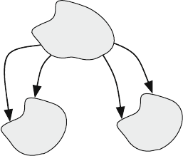
of two or more closed states. Figure 5.4 shows a reducible Markov chain with two
sets of closed states. If the system is in the transient state T , it can move to either
sets of closed states, C
1
or C
2
. However, if the system is in state C
1
, it cannot move
to T or C
2
. Similarly, if the system is in state C
2
, it can not move to T or C
1
.
Assume the transition matrix is given by the canonic form
P =
⎡
⎣
C
1
0A
1
0C
2
A
2
00T
⎤
⎦
(5.23)
5.8 Reducible Composite Markov Chains at Steady-State 165
Transient
State T
Closed
State
C
1
Closed
State
C
2
Fig. 5.4 A reducible Markov chain with two sets of closed states
where
C
1
and C
2
= square column stochastic matrices
A
1
and A
2
= rectangular nonnegative matrices
T = square column substochastic matrix
It is easy to verify that the steady-state transition matrix for such a system will be
P
∞
=
⎡
⎣
C
1
0Y
1
0C
1
Y
2
000
⎤
⎦
(5.24)
where
C
1
= C
∞
1
(5.25)
C
1
= C
∞
2
(5.26)
Y
1
= C
1
A
1
(
I −T
)
−1
(5.27)
Y
2
= C
1
A
2
(
I −T
)
−1
(5.28)
Essentially, C
1
is the matrix that is associated with λ = 1 in the expansion of C
1
in terms of its eigenvalues. The same also applies to C
1
, which is the matrix that is
associated with λ = 1 in the expansion of C
2
in terms of its eigenvalues.
We observe that each column of matrix Y
1
is a scaled copy of the columns of
C
1
. Also, the sum of each column of Y
1
is lesser than one. We can make the same
observations about matrix Y
2
.
Example 5.8 The given transition matrix corresponds to a composite reducible
Markov chain.
P =
⎡
⎢
⎢
⎢
⎢
⎢
⎢
⎣
0.50.3000.10.4
0.50.7000.30.1
000.20.70.10.2
000.80.30.10.1
00000.10.2
00000.30
⎤
⎥
⎥
⎥
⎥
⎥
⎥
⎦
166 5 Reducible Markov Chains
Find its eigenvalues and eigenvectors then find the steady-state distribution
vector.
The components of the transition matrix are
C
1
=
0.50.3
0.50.7
C
2
=
0.20.7
0.80.3
A
1
=
0.20.4
0.20.1
A
2
=
0.10.2
0.10.1
T =
0.10.2
0.30
The steady-state value of C
1
is
C
1
=
0.375 0.375
0.625 0.625
The matrix Y
1
has the value
Y
1
= C
1
A
1
(
I −T
)
−1
=
0.2455 0.2366
0.4092 0.3943
The steady-state value of C
2
is
C
1
=
0.4667 0.4667
0.5333 0.5333
The matrix Y
2
has the value
Y
2
= C
1
A
2
(
I −T
)
−1
=
0.1611 0.1722
0.1841 0.1968
Thus the steady-state value of P is
P
∞
=
⎡
⎢
⎢
⎢
⎢
⎢
⎢
⎣
0.375 0.375 0 0 0.2455 0.2366
0.625 0.625 0 0 0.4092 0.3943
000.4667 0.4667 0.1611 0.1722
000.5333 0.5333 0.1841 0.1968
000000
000000
⎤
⎥
⎥
⎥
⎥
⎥
⎥
⎦