Gebali F. Analysis Of Computer And Communication Networks
Подождите немного. Документ загружается.

126 4 Markov Chains at Equilibrium
2. The eigenvector technique (2) is used when P is expressed numerically and its
size is reasonable so that any mathematical package could easily find the eigen-
vector. Some communication systems are described by a small 2 × 2 transition
matrix and it is instructive to get a closed-form expression for s. We shall see this
for the case of packet generators.
3. The difference equations technique (3) is used when P is banded with few subdi-
agonals. Again, many communication systems have banded transition matrices.
We shall see many examples throughout this book about such systems.
4. The z-transform technique (4) is used when P is lower triangular or lower
Hessenberg such that each diagonal has identical elements. Again, some commu-
nication systems have this structure and we will discuss many of them throughout
this book.
5. The direct technique (5) is used when P is expressed numerically and P has no
particular structure. Furthermore, the size of P is not too large such that round-
ing or truncation noise is insignificant. Direct techniques produce results with
accuracies dependent on the machine precision and the number of calculations
involved.
6. The iterative numerical technique (6) is used when P is expressed numerically
and P has no particular structure. The size of P has little effect on truncation
noise because iterative techniques produce results with accuracies that depend
only on the machine precision and independent of the number of calculations
involved.
7. The iterative technique (7) for expressing the states of P in terms of other states
is illustrated in Section 9.3.2 on page 312.
We illustrate these approaches in the following sections.
4.6 Finding s Using Eigenvector Approach
In this case we are interested in finding the eigenvector s which satisfies the
condition
Ps= s (4.4)
MATLAB and other mathematical packages such as Maple and Mathematica
have commands for finding that eigenvector as is explained in Appendix E. This
technique is useful only if P is expressed numerically. Nowadays, those mathemat-
ical packages can also do symbolic computations and can produce an answer for s
when P is expressed in symbols. However, symbolic computations demand that the
the size of P must be small, in the range of 2–5, at the most to get any useful data.
Having found a numeric or symbolic answer, we must normalize s to ensure that
i
s
i
= 1 (4.5)
4.7 Finding s Using Difference Equations 127
Example 4.2 Find the steady-state distribution vector for the following transition
matrix.
P =
⎡
⎣
0.80.70.5
0.15 0.20.3
0.05 0.10.2
⎤
⎦
We use MATLAB to find the eigenvectors and eigenvalues for P :
s
1
=
0.9726 0.2153 .0877
t
↔λ
1
= 1
s
2
=
0.8165 −0.4882 −0.4082
t
↔λ
2
= 0.2
s
3
=
0.5345 −0.8018 0.2673
t
↔λ
3
= 0
The steady-state distribution vector s corresponds to s
1
and we have to normalize
it. We have
i
s
i
= 1.2756
Dividing s
1
by this value we get the steady-state distribution vector as
s
1
=
0.7625 0.1688 0.0687
t
4.7 Finding s Using Difference Equations
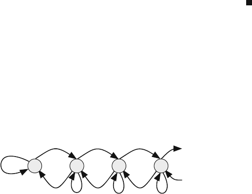
This technique for finding s is useful only when the state transition matrix P is
banded. Consider the Markov chain representing a simple discrete-time birth–death
process whose state transition diagram is shown in Fig. 4.1. For example, each state
might correspond to the number of packets in a buffer whose size grows by one
or decreases by one at each time step. The resulting state transition matrix P is
tridiagonal with each subdiagonal composed of identical elements.
0 1
2 3
f
0
bc
fff
ad ad ad ad
bc bc bc
Fig. 4.1 State transition diagram for a discrete-time birth–death Markov chain
128 4 Markov Chains at Equilibrium
We make the following assumptions for the Markov chain.
1. The state of the Markov chain corresponds to the number of packets in the buffer
or queue. s
i
is the probability that i packets are in the buffer.
2. The size of the buffer or queue is assumed unrestricted.
3. The probability of a packet arriving to the system is a at a particular time, and
the probability that a packet does not arrive is b = 1 −a.
4. The probability of a packet departing the system is c at a particular time, and the
probability that a packet does not depart is d = 1 −c.
5. When a packet arrives it could be serviced at the same time step and it could
leave the queue, at that time step, with probability c.
From the transition diagram, we write the state transition matrix as
P =
⎡
⎢
⎢
⎢
⎢
⎢
⎣
f
0
bc 00···
ad f bc 0 ···
0 ad f bc ···
00ad f ···
.
.
.
.
.
.
.
.
.
.
.
.
.
.
.
⎤
⎥
⎥
⎥
⎥
⎥
⎦
(4.6)
where f
0
= ac +b and f = ac +bd. For example, starting with state 1, the system
goes to state 0 when a packet does not arrive and the packet that was in the buffer
departs. This is represented by the term bc at location (1,2) of the matrix.
Using this matrix, or the transition diagram, we can arrive at difference equa-
tions relating the equilibrium distribution vector components as follows. We start
by writing the equilibrium equation
Ps= s (4.7)
Equating corresponding elements on both sides of the equation, we get the fol-
lowing equations.
ad s
0
−bc s
1
= 0 (4.8)
ad s
0
− gs
1
+bc s
2
= 0 (4.9)
ad s
i−1
− gs
i
+bc s
i+1
= 0 i > 0 (4.10)
where g = 1 − f and s
i
is the ith component of the state vector s which is equal
to the probability that the system is in state i. Appendix B gives techniques for
solving such difference equations. However, we show here a simple method based
on iterations. From (4.8), (4.9), and (4.10) we can write the expressions

4.7 Finding s Using Difference Equations 129
s
1
=
ad
bc
s
0
s
2
=
ad
bc
2
s
0
s
3
=
ad
bc
3
s
0
and in general
s
i
=
ad
bc
i
s
0
i ≥ 0 (4.11)
It is more convenient to write s
i
in the form
s
i
= ρ
i
s
0
i ≥ 0 (4.12)
where
ρ =
ad
bc
< 1 (4.13)
In that sense ρ can be thought of as distribution index that dictates the magnitude
of the distribution vector components. The complete solution is obtained from the
above equations, plus the condition
∞
i=0
s
i
= 1 (4.14)
By substituting the expressions for each s
i
in the above equation, we get
s
0
∞
i=0
ρ
i
= 1 (4.15)
Thus we obtain
s
0
1 −ρ
= 1 (4.16)
from which we obtain the probability that the system is in state 0 as
s
0
= 1 −ρ (4.17)
and the components of the equilibrium distribution vector is given from (4.12) by
s
i
= (1 −ρ)ρ
i
i ≥ 0 (4.18)

130 4 Markov Chains at Equilibrium
For the system to be stable we must have ρ<1. If we are interested in situations
where ρ ≥ 1 then we must deal with finite-sized systems where the highest state
could be s
B
and the system could exist in one of B + 1 states only. This situation
will be treated more fully in Section 7.6 on page 233.
Example 4.3 Consider the transition matrix for the discrete-time birth–death pro-
cess that describes single-arrival, single-departure queue with the following param-
eters a = 0.4 and c = 0.6. Construct the transition matrix and find the equilibrium
distribution vector.
The transition matrix becomes
P =
⎡
⎢
⎢
⎢
⎢
⎢
⎣
0.84 0.36 0 0 ···
0.16 0.48 0.36 0 ···
00.16 0.48 0.36 ···
000.16 0.48 ···
.
.
.
.
.
.
.
.
.
.
.
.
.
.
.
⎤
⎥
⎥
⎥
⎥
⎥
⎦
Using (4.13), the distribution index is equal to
ρ = 0.4444
From (4.17) we have
s
0
= 0.5556
and from (4.18) we have
s
i
= (1 −ρ)ρ
i
= (0.5556) ×0.4444
i
The distribution vector at steady state is
s =
0.5556 0.2469 0.1097 0.0488 0.0217 ···
t
4.8 Finding s Using Z-Transform
This technique is useful to find the steady-state distribution vector s only if the
state transition matrix P is lower Hessenberg such that elements on one diagonal
are mostly identical. This last restriction will result in difference equations with
constant coefficients for most of the elements of s. This type of transition matrix
occurs naturally in multiple-arrival, single-departure (M
m
/M/1) queues. This queue
will be discussed in complete detail in Section 7.6 on page 233.
4.8 Finding s Using Z-Transform 131
Let us consider a Markov chain where we can move from state j to any state i
where i ≥ j − 1. This system corresponds to a buffer, or queue, whose size can
increase by more than one due to multiple packet arrivals at any time, but the size of
the queue can only decrease by one due to the presence of a single server. Assume
the probability of K arrivals at instant n is given by
p(K arrivals) = a
K
K = 0, 1, 2, ... (4.19)
for all time instants n = 0, 1, 2,...Assume that the probability that a packet is able
to leave the queue is c and the probability that it is not able to leave the queue is
d = 1 −c.
The condition for the stability of the system is
∞
K=0
Ka
K
< c (4.20)
which indicates that the average number of arrivals at a given time is less than the
average number of departures from the system. The state transition matrix will be
lower Hessenberg:
P =
⎡
⎢
⎢
⎢
⎢
⎢
⎣
a
0
b
0
00···
a
1
b
1
b
0
0 ···
a
2
b
2
b
1
b
0
···
a
3
b
3
b
2
b
1
···
.
.
.
.
.
.
.
.
.
.
.
.
.
.
.
⎤
⎥
⎥
⎥
⎥
⎥
⎦
(4.21)
where b
i
= a
i
c +a
i−1
d and we assumed
a
i
= 0 when i < 0
Note that the sum of each column is unity, as required from the definition of a
Markov chain transition matrix. At equilibrium we have
Ps= s (4.22)
The general expression for the equilibrium equations for the states is given by
the i-th term in the above equation
s
i
= a
i
s
0
+
i+1
j=1
b
i−j+1
s
j
(4.23)
This analysis is a modified and simpler version of the one given in reference [1].
Define the z-transform for the state transition probabilities a
i
and b
i
as
132 4 Markov Chains at Equilibrium
A(z) =
∞
i=0
a
i
z
−i
(4.24)
B(z) =
∞
i=0
b
i
z
−i
(4.25)
One observation worth mentioning here for later use is that since all entries in
the transition matrix are positive, all the coefficients of A(z) and B(z) are positive.
We define the z-transform for the equilibrium distribution vector s as
S(z) =
∞
i=0
s
i
z
−i
(4.26)
where s
i
are the components of the distribution vector. From (4.23) we can write
S(z) = s
0
∞
i=0
a
i
z
−i
+
∞
i=0
i+1
j=1
b
i−j+1
s
j
z
−i
(4.27)
= s
0
A(z) +
∞
i=0
∞
j=1
b
i−j+1
s
j
z
−i
(4.28)
we were able to change the upper limit for j, in the above equation, by assuming
b
i
= 0 when i < 0 (4.29)
Now we change the order of the summation
S(z) = s
0
A(z) +
∞
j=1
∞
i=0
b
i−j+1
s
j
z
−i
(4.30)
Making use of the assumption in (4.29), we can change the limits of the summa-
tion for i
S(z) = s
0
A(z) +
⎡
⎣
∞
j=1
s
j
z
−j
⎤
⎦
×
∞
i=j−1
b
i−j+1
z
−(i−j)
(4.31)
We make use of the definition of S(z) to change the term in the square brackets:
S(z) = s
0
A(z) +
[
S(z) −s
0
]
×
∞
i=j−1
b
i−j+1
z
−(i−j)
(4.32)
We now change the summation symbol i by using the new variable m = i − j +1

4.8 Finding s Using Z-Transform 133
S(z) =s
0
A(z) +
[
S(z) −s
0
]
× z
∞
m=0
b
m
z
−m
=s
0
A(z) + z
[
S(z) −s
0
]
B(z) (4.33)
We finally get
S(z) = s
0
×
z
−1
A(z) − B(z)
z
−1
− B(z)
(4.34)
Below we show how we can obtain a numerical value for s
0
. Assuming for the
moment that s
0
is found, MATLAB allows us to find the inverse z-transform of
S(z) using the command RESIDUE(a,b) where a and b are the coefficients of
A(z) and B(z), respectively, in descending powers of z
−1
. The function RESIDUE
returns the column vectors r, p, and c which give the residues, poles, and direct
terms, respectively.
The solution for s
i
is given by the expression
s
i
= c
i
+
m
j=1
r
j
(p
j
)
(i−1)
i > 0 (4.35)
where m is the number of elements in r or p vectors. The examples below show
how this procedure is done.
When z = 1, the z-transforms for s, a
i
, and b
i
are
S(1) =
∞
j=1
s
j
= 1 (4.36)
A(1) = B(1) = 1 (4.37)
Thus we can put z = 1 in (4.34) and use L’Hospital’s rule to get
s
0
=
1 + B
(1)
1 + B
(1) − A
(1)
(4.38)
where
A
(1) =
dA(z)
dz
z=1
< 0 (4.39)
B
(1) =
dB(z)
dz
z=1
< 0 (4.40)
Since all the coefficients of A(z) and B(z) are positive, all the coefficients of A
and B
are negative and the two numbers A
(1) and B
(1) are smaller than zero. As a
134 4 Markov Chains at Equilibrium
result of this observation, it is guaranteed that s
0
< 1 as expected for the probability
that the queue is empty.
We should note that the term −A
(1) represents the average number of packet
arrivals per time step when the queue is empty. Similarly, −B
(1) represents the
average number of packet arrivals per time step when the queue is not empty.
Having found a numerical value for s
0
, we use (4.34) to obtain the inverse z-
transform of S(z) and get expressions for the steady-state distribution vector
s =
s
0
s
1
s
2
···
(4.41)
Example 4.4 Use the z-transform technique to find the equilibrium distribution vec-
tor for the Markov chain whose transition matrix is
P =
⎡
⎢
⎢
⎢
⎢
⎢
⎣
0.84 0.36 0 0 ···
0.16 0.48 0.36 0 ···
00.16 0.48 0.36 ···
000.16 0.48 ···
.
.
.
.
.
.
.
.
.
.
.
.
.
.
.
⎤
⎥
⎥
⎥
⎥
⎥
⎦
The transition probabilities are given by
a
0
= 0.84
a
1
= 0.16
a
i
= 0 when i > 1
b
0
= 0.36
b
1
= 0.48
b
2
= 0.16
b
i
= 0 when i > 2
We have the z-transforms of A(z) and B(z)as
A(z) = 0.84 +0.16z
−1
B(z) = 0.36 +0.48z
−1
+0.16z
−2
Differentiation of the above two expressions gives
A(z)
=−0.16z
−2
B(z)
=−0.48z
−2
−0.32z
−3
By substituting z
−1
= 1 in the above expressions, we get

4.8 Finding s Using Z-Transform 135
A(1)
=−0.16
B(1)
=−0.8
By using (4.38) we get the probability that the queue is empty
s
0
=
1 + B
(1)
1 + B
(1) − A
(1)
= 0.5556
From (4.34) we can write
S(z) =
0.2 −0.2z
−1
0.36 −0.52z
−1
+0.16z
−2
We can convert the polynomial expression for S(z) into a partial-fraction expan-
sion (residues) using the MATLAB command RESIDUE:
b = [0.2, -0.2]; a = [0.36,
-0.52, 0.16]; [r,p,c] = residue(b,a)
r=
0.0000
0.2469
p=
1.0000
0.4444
c=
0.5556
where the column vectors r, p, and c give the residues, poles, and direct terms,
respectively. Thus we have
s
0
= c = 0.5555
which confirms the value obtained earlier. For i ≥ 1wehave
s
i
=
j
r
j
p
j
i−1
Thus the distribution vector at steady state is given by
s =
0.5556 0.2469 0.1097 0.0488 0.0217 ···
t
Note that this is the same distribution vector that was obtained for the same ma-
trix using the difference equations approach in Example 4.3.
As as a check, we generated the first 50 components of s and ensured that their
sum equals unity.