Durst F. Fluid Mechanics: An Introduction to the Theory of Fluid Flows

Подождите немного. Документ загружается.

492 16 Flows of Large Reynolds Numbers

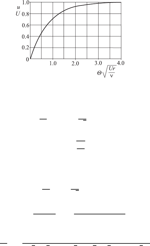
Fig. 16.15 Velocity distribution in a laminar boundary layer forming at the walls

of a converging channel

or rewritten:



(η)=

=3tanh



√

+1.146



− 2. (16.152)

Introducing also Θ = y/x and

Q = rUα, one can rewrite η as:

η = Θ

(16.153)

and the velocity distribution shown in Fig. 16.15 results for the boundary

layer at the walls of a converging, plane, two-dimensional channel ﬂow.

The above-obtained relationship (16.152):

αx

tanh



√

+1.146



− 2 (16.154)

canalsobewrittenas:

tanh

[Z]=1−

cosh

[Z]

=1−

(exp[Z]+exp[−Z])

. (16.155)

This can be inserted to yield the velocity distribution:

αx

1 −

(

√

2) exp(η/

√

2) + (

√

3 −

√

2) exp(−η/

√

(16.156)

References

16.1. G. K. Batchelor: “An Introduction to Fluid Dynamics”, Cambridge University

Press, Cambridge (1967)

16.2. B. A. Boley and M. B. Friedman: On the Viscous Flow Around the Leading

Edge of a Flat Plate, JASS 26, 453–454 (1959)

References 493

16.3. G. F. Carrier and C. C. Lin: On the Nature of the Boundary Layer Near the

Leading Edge of a Flat Plate, Q. Appl. Math. VI, 63–68 (1948)

16.4. D. Pnueli and C. Gutﬁnger: “Fluid Mechanics”, Cambridge University Press,

Cambridge (1992)

16.5. H. Schlichting: “Boundary Layer Theory”, 6th edition, McGraw-Hill, New York

(1968)

16.6. F. S. Sherman: “Viscous Flow”, McGraw-Hill, Singapore (1990)

16.7. J. M. Shi, F. Durst and M. Breuer: Matching Asymptotic Computation of the

Viscous Flow Around the Leading Edge of a Flat Plate, in preparation.

16.8. F. Durst: “Str¨omungslehre – Einf¨uhrung in die Theorie der Str¨omungen”, 4,

Springer, Berlin Heidelberg New York (1996)

16.9. C. S. Yih: “Fluid Mechanics – A Concise Introduction to the Theory”, West

River Press, Ann Arbor, MI (1979)

Chapter 17

Unstable Flows and Laminar-Turbulent

Transition

17.1 General Considerations

It is common practice to categorize ﬂows as laminar or turbulent, i.e. to

employ a special state of the ﬂow to perform a subdivision: into laminar ﬂows,

i.e. in such ﬂows in which the momentum, heat and mass transport processes

are molecular dependent, and into such ﬂows in which turbulence-dependent

transport processes occur in addition. For the considerations presented in

this chapter, a further subdivision is appropriate, so that grouping into four

sub-groups is made:

• Stable Laminar Flows. A laminar ﬂow may fulﬁll all requirements of the

basic equations of ﬂuid mechanics. It may also satisfy the initial and

boundary conditions characteristic for the ﬂow. Yet it must not represent

a solution such as one ﬁnds in corresponding experimental investigations.

Disturbances of the ﬂow, as always occur in experiments, are often not

considered in solutions of the basic equations governing ﬂuid ﬂows. Only

such laminar ﬂows that prove stable towards disturbances that act from

the outside, i.e. attenuate the imposed disturbances, are deﬁned as stable

laminar ﬂows.

• Unstable Laminar Flows. A laminar ﬂow is considered unstable when

disturbances introduced into it are ampliﬁed, but a certain “regularity”

in the excited disturbance is maintained, i.e. due to the disturbance

the investigated ﬂow merges into a new laminar ﬂow state. If this “new

laminar ﬂow state” is stable towards newly introduced disturbances, we

have a bifurcation of the laminar ﬂow. Here it is important to understand

that the ﬂow occurring after the imposed disturbance can be stationary

or non-stationary.

• Transitional Flows. When the disturbances introduced in a laminar

ﬂow are ampliﬁed and result in ﬂows that appear orderly in parts, but

show also temporarily and/or spatially irregular ﬂuctuations of all ﬂow

quantities, we speak of a transitional ﬂow state. Intermittent laminar and

495

496 17 Unstable Flows

turbulent ﬂow states occur, i.e. phases occur in the ﬂow in which the ﬂow

is laminar and phases in which the ﬂow shows turbulent characteristics.

Flows that are in a transitional state still show clear characteristics that

depend on the imposed disturbances.

• Turbulent Flows. It is now easily possible to imagine, on the basis of

the considerations presented above, that disturbances are introduced

into ﬂows to such an extent that ﬂuid motions result from them that

are “out of control.” Such turbulent ﬂuctuations of all ﬂow quantities

are superimposed on corresponding mean ﬂow quantities and are char-

acterized by high non-stationarity and by high three-dimensionality.

Turbulence-dependent transport processes of momentum, heat and mass

are superimposed on the molecular-dependent transport process. A closed

treatment of turbulent transport processes is at present only possible for

small Reynolds numbers (Re ≤ 40,000) by employing numerical com-

putation procedures. The treatment of turbulent ﬂows at high Reynolds

numbers remains a problem of ﬂuid mechanics that has not been solved.

In the preceding chapters, ﬂows were investigated that are assumed to be

stable, i.e. without concrete proof it was assumed that disturbances which are

introduced into the ﬂow are damped out by viscosity. In order to understand

now the causes of stable laminar ﬂows, i.e. the causes of the attenuation of

disturbances by viscosity, the simpliﬁed one-dimensional momentum equation

is considered:

∂U

∂t

= µ

∂

∂x

. (17.1)

When applying this to a ﬂow with a constant ﬂow velocity U

,onwhich

a disturbance with amplitude u

is superimposed, the following equation

applies for the total velocity ﬁeld:

= U

+ u

sin



2π



with U

= constant. (17.2)

On now forming the temporal derivative (∂U

/∂t) and the spatial derivative

(∂

/∂x

), one obtains from (17.2) the following diﬀerential equation for

the disturbance. It indicates how the temporal change of the amplitude of

the imposed ﬂuctuations behaves in time:

= −ν

4π

. (17.3)

This diﬀerential equation can be solved by separation of the variables. Thus,

for the initial condition u

=(u

)

,forthetimet ≥ 0 the following solution

can be derived:

(t)=(u

)

exp



−ν

4π



. (17.4)

This solution makes it clear that the viscosity terms in the momentum equa-

tions can be considered to lead to attenuations of imposed disturbances, i.e.

disturbances which are introduced into a laminar ﬂow ﬁeld will be damped

17.1 General Considerations 497

due to the viscosity of the ﬂuid. As expressed by (17.4), the attenuation of

short-wave disturbances, i.e. disturbances with small λ values, turns out to

be stronger, so that these receive stronger damping in the course of time. It

is this attenuation eﬀect, caused by the viscosity of a ﬂuid, which ensures

that many laminar ﬂows possess high stability. This means that they show

strong resistance against external disturbances.

As concerns the possible mechanisms of ampliﬁcation of disturbances,

these can be manifold and some are discussed in an introductory way in sub-

sequent sections. Generally it can be said, however, that gradients of ﬂow

and/or ﬂuid properties can be stated as causes of ampliﬁcation. When they

act on introduced disturbances such that an exponential excitation takes

place, the latter can be described as follows:

=(u

)

exp(αt). (17.5)

When a viscosity-dependent attenuation exists at the same time, the temporal

development of the amplitude of a disturbance can be stated in a simpliﬁed

way, and the following net result can be assumed to be valid:

=(u

)

exp [(α − β)t] . (17.6)

When the viscosity-dependent attenuation term β proves to be larger than

the ampliﬁcation-caused term α, i.e. β>α, we have a stable laminar ﬂow.

When, on the other hand, the ampliﬁcation term α dominates, i.e. α>β,

we have an unstable ﬂow. This means that the ﬂow ﬁeld determined from

the Navier–Stokes equations for given initial and boundary conditions will

not form in practice. Due to the above-postulated exponential increase of the

disturbance introduced into the ﬂow, a transition into a turbulent ﬂow is to

be expected. When the excitation takes place in another, non-exponential

form, other unstable ﬂow states, as mentioned in the above points, can form.

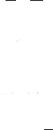
To make clear now what is to be understood by a stable laminar ﬂow state,

reference is made to the backward-facing, double-sided step ﬂow, which is

illustrated in Fig. 17.1. It shows a symmetrical solution for Re ≤ 200. When

imposing temporal disturbances on these ﬂows, the temporal change of the

separation lengths x

, shown in Fig. 17.1, indicates that, after abandoning

the imposed disturbances, the separation and reattachment lengths, that are

characteristic for the step ﬂow, are attained again. The ﬂow is thus, for the

investigated Reynolds number, stable towards the imposed disturbances. At

higher Reynolds numbers, i.e. for Re ≥ 200, this stability no longer exists.

The ﬂow abandons its symmetry, and two separate regions of diﬀerent lengths

and shapes occur.

For further explanations of the processes that take place with unstable

laminar ﬂows, reference is made to the ﬂow through a rectangular channel.

The latter is characterized by secondary ﬂows as shown in Fig. 17.2. These

so-called secondary ﬂows represent ﬂuid motions in a plane vertical to the

main ﬂow. Depending on the Reynolds number, a certain secondary ﬂow

pattern develops as the so-called bifurcation diagram demonstrates, which

498 17 Unstable Flows

(a)

(b)

(c)

Stable flow region

Bifurcation point

Fig. 17.1 (A) Stability of double-sided step ﬂow (sudden expansion): (a)sym-

metrical solution (unstable); (b) asymmetric solution (stable solution of the ﬁrst

bifurcation); (c) asymmetric solution (unstable solution of the second bifurcation).

(B) Bifurcation diagram for a ﬂow with sudden extension

Fig. 17.2 Pattern of the secondary ﬂow in a rectangular channel and corresponding

bifurcation diagram

is also shown in Fig. 17.2. Detailed numerical investigations show, however,

that certain patterns of secondary ﬂow can only be obtained by imposed

disturbances that are well directed.

17.1 General Considerations 499

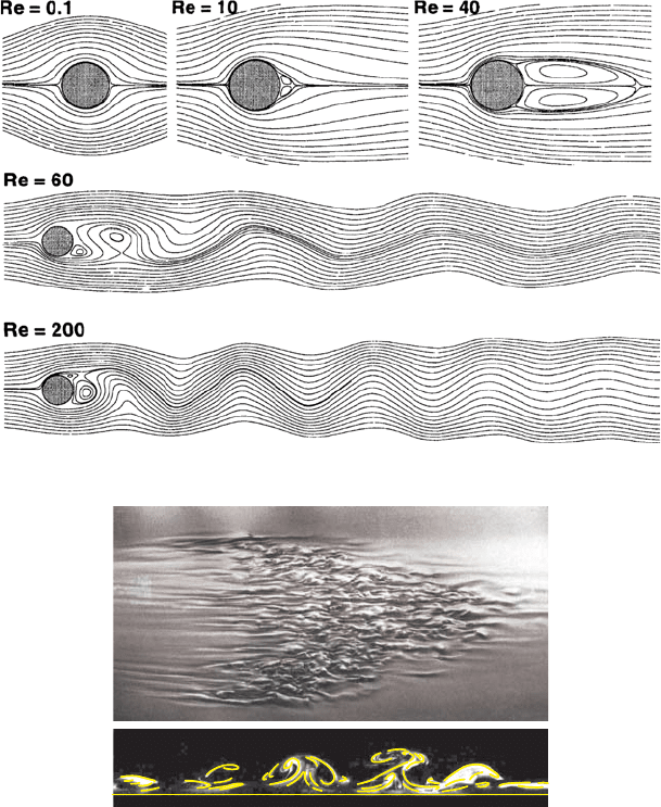
Another possibility of bifurcation of an unstable laminar ﬂow is given in

Fig. 17.3. This ﬁgure shows that the laminar ﬂow around a cylinder posseses

a symmetry of the ﬂow ﬁeld for small Re.ForRe ≥ 46 the “symmetry” is

broken. A non-stationary vortex ﬂow (Hopf bifurcation) develops with alter-

nating vortices relieving one another. In the wake of the cylinder, the so-called

Karman vortex street results as the form of the laminar ﬂow around a cylinder

which proves to be a stable ﬂow form for Re > 46.

To illustrate a transitional ﬂow, reference is made to Fig. 17.4, in which a

region of turbulent ﬂow is shown that is embedded in a laminar plate ﬂow.

It can clearly be seen that the turbulence-dependent ﬂow disturbances are

Fig. 17.3 Flow forms of the laminar ﬂows around a cylinder

Fig. 17.4 Turbulent spot to illustrate the transitional, laminar-to-turbulent ﬂow

state of a ﬂow; see van Dyke [17.1]

500 17 Unstable Flows

spatially and temporally limited. Likewise, a certain, still clearly distinctive

structure of the ﬂow can be recognized. All of these are clear characteristics

of ﬂows that are in a transitional, laminar-to-turbulent ﬂow state.

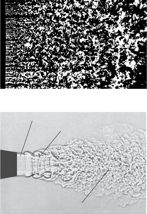
As a turbulent state of a ﬂow, the photograph illustrates a grid wake

ﬂow, which is made visible by introduced smoke. The “ﬁlaments” of smoke,

introduced near the grid, are structured by the turbulent ﬂuid motions and

form a typical picture of an almost isotropic ﬂow ﬁeld. By isotropy of a ﬂow a

local property is understood, namely the independence of the mean properties

of the ﬂow of considered directions (Fig. 17.5).

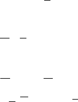
That the ﬂow states described above can occur within one ﬂow region is

illustrated in Fig. 17.6. This ﬁgure shows an open jet coming out of a nozzle

Fig. 17.5 Turbulent grid wake ﬂow: making turbulent ﬂow properties visible by

introduced smoke; see van Dyke [17.1]

Laminar flow

Transitional flow

Turbulent flow

Fig. 17.6 Subsonic open jet with areas of laminar, transitional and turbulent ﬂow;

see van Dyke [17.1]

17.2 Causes of Flow Instabilities 501

which shows laminar ﬂow behavior in the immediate vicinity of the nozzle.

The laminar ﬂow becomes unstable and leads to a laminar-to-turbulent tran-

sition behavior, before further downstream the ﬂow becomes completely

turbulent. For the last-named ﬂow region it is characteristic that no dis-

tinctively coherent ﬂow structures can be recognized any more. This makes

it clear that the transitional ﬂow behavior can occur in parts of ﬂows. In

front of these transitional sub-domains the ﬂow is laminar and behind these

domains (looked at in the ﬂow direction) the ﬂow is turbulent.

17.2 Causes of Flow Instabilities

Flow instabilities show features that are manifold, and there is an extensive

literature available on their causes and on the resultant ﬂow structures that

can be observed. It shall be the task here to discuss some of the causes that

occur and the resultant ﬂow phenomena. The chapter tries to give an in-

troduction to the considerations that have to be carried out to investigate

ﬂow instabilities theoretically. The methods employed in the considerations

are also part of the presentations, but they are limited to selected examples.

They were chosen, however, such that they clearly illustrate the full attraction

of ﬂuid-mechanical investigations of unstable ﬂows. Hence, the aim of the pre-

sented material is to ensure that students of ﬂuid mechanics receive an early

introduction to the broad (but also very specialized) ﬁeld of non-stationary

ﬂow investigations, and that they are made familiar with the available solu-

tion methods. Here, it is important always to take the below-mentioned steps

towards a solution of the posed instability problems:

(a) Determine the main ﬂow ﬁeld as an analytical or numerical solution of the

Navier–Stokes equations and for the boundary conditions determining

the ﬂow problem.

(b) Utilize the basic equations to derive equations to treat ﬂow disturbances.

Carry out considerations for small amplitudes of the disturbances, i.e.

use the linearized equations to compute the disturbance. In this way,

linear, partial diﬀerential equations result and have to be treated for the

disturbances of all ﬂow quantities to be considered.

tem for given disturbances, in order to investigate the increase or decrease

in the amplitude of the disturbances in space and time.

(d) The linear, partial diﬀerential equation system can be solved, to some

extent, for the general propagations of disturbances. Solutions do not

exist for all disturbances, so that one is often forced to carry out further

simpliﬁcations. The derivation of the Orr–Sommerfeld equation results

from such a simpliﬁcation.

502 17 Unstable Flows

(e) Finally, interpretations of the results obtained are needed for deciding

the ranges of parameter values for stable or unstable, laminar ﬂows.

Steps (a)–(e) are shown in parts of the subsequent derivations.

17.2.1 Stability of Atmospheric Temperature Layers

In Chap. 6, the pressure distribution in the atmosphere was considered

for very diﬀerent temperature distributions, e.g. also for the following

temperature distribution:

T (x

)=T



1 −



, (17.7)

which states a linear temperature decrease with increasing height above sea

level. In this relationship γ = T

/c is the (existing) temperature gradient:

= constant. (17.8)

For the temperature distribution in the atmosphere, given by (17.7), the

corresponding pressure distribution could be found by integration of the

following equation:

= −gρ = −

P (17.9)

resulting in

P = P



1 −



= P

− γx

)

Rγ

. (17.10)

In the considerations in Chap. 6, it was indirectly assumed that the chosen

temperature distribution is stable, i.e. introduced disturbances leave the im-

posed temperature distribution undisturbed. Here, the extent to which this

holds true will be investigated, i.e. up to what temperature layer the imposed

temperature gradient is stable.

To be able to carry out the required stability considerations, a ﬂuid el-

ement is considered which is deﬂected upwards for a short time. Here the

deﬂection of the ﬂuid element is considered under adiabatic conditions. When

the deﬂection leads to a buoyancy force on the ﬂuid element, increasing the

induced deﬂection, the temperature distribution is considered to be unsta-

ble. When the deﬂected ﬂuid element experiences a restoring force, which is

directed such that a reduction of the deﬂection takes place, we have a stable

temperature distribution in the considered atmosphere (Fig. 17.7).

Taking the temperature T



as the temperature of a ﬂuid particle which

experiences an adiabatic upward movement from z to z +dz, the following

relationship holds under adiabatic conditions: