Durst F. Fluid Mechanics: An Introduction to the Theory of Fluid Flows

Подождите немного. Документ загружается.

482 16 Flows of Large Reynolds Numbers

( U )

Velocity profiles at

different

-position

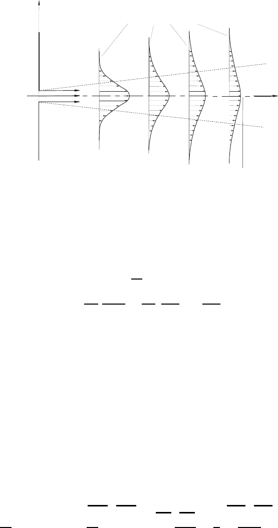
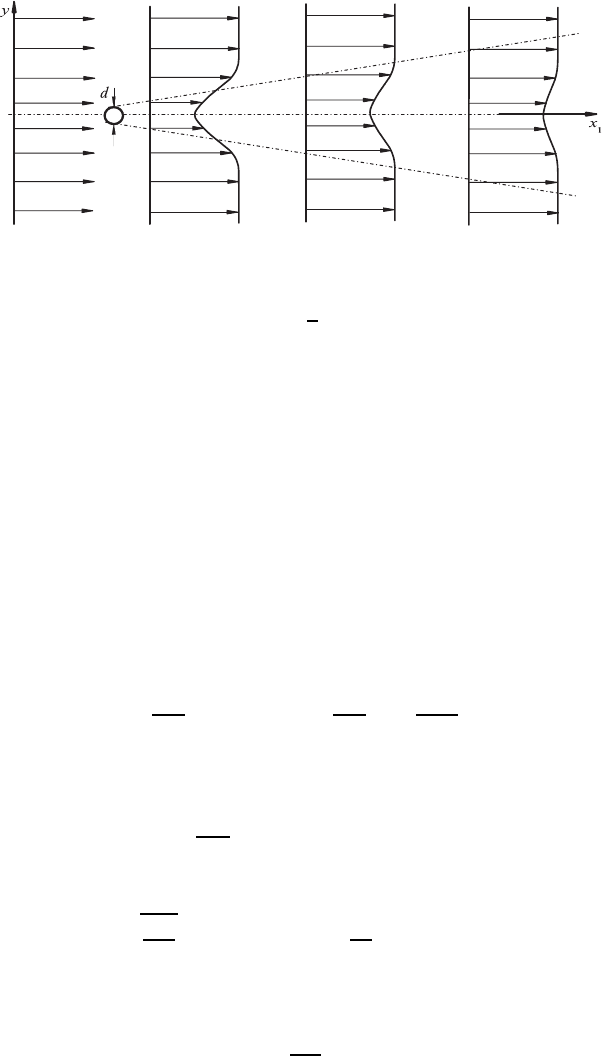
Fig. 16.10 Sketch of the considered plane, two-dimensional laminar free jet

Below a two-dimensional free jet is considered, which can be generated

in the plane x = 0, by a ﬂow from a narrow slit located in the x – y plane.

The jet propagates in the x-direction and the propagation is such, that the

x-axis is the symmetry axis. As the propagation of the jet occurring in the

y-direction is small in comparison with the propagation in the ﬂow direction

and as, moreover, only stationary main ﬂow conditions will be considered,

the boundary-layer equation for

=0canbeemployedtostudytheﬂow:

∂Ψ

∂y

∂

∂x∂y

−

∂Ψ

∂x

∂

∂y

= ν

∂

∂y

. (16.81)

This is again the boundary-layer equation for Ψ as it was employed in the

case of the ﬂow along a ﬂat plate and also when the plane shear layer was

considered. The diﬀerence from the plate boundary-layer ﬂow occurs due to

the boundary conditions, which for the free jet ﬂow are as follows:

y =0: U

=0and(∂U

/∂y)=0, as is the symmetry axis,

y = ∞ : U

→ 0, as there is no background ﬂow.

(16.82)

For the free jet, the total momentum can be derived as:

ges

+∞

−∞

ρU

dy =2

+∞

ρU

dy =2ρ (U

)

b. (16.83)

The momentum is constant along the x-axis. This follows from (16.68), which

holds for the free jet as given below:

+∞

dy −U

∞

  

+∞

dy −

  

∞

  

+∞

∂

∂y

dy (16.84)

16.6 The Plane, Two-Dimensional, Laminar Free Jet 483

so that one can derive

+∞

dy =0 ; I

ges

+∞

ρU

dy = constant. (16.85)

For deriving the similarity solution for the free jet ﬂow, the boundary-layer

equation can be solved with the following ansatzes:

η = x

y and Ψ = x

f(η). (16.86)

From this the diﬀerent terms in the boundary layer equation can be expressed

as follows in terms of the introduced quantities η and Ψ:

∂Ψ

∂y

= x

(α+β)



, (16.87)

= −

∂Ψ

∂x

= −x

(β−1)

(αηf



+ βf) , (16.88)

∂U

∂y

∂

∂y

= x

(2α+β)



, (16.89)

∂

∂x∂y

= x

(α+β−1)

(αηf



+ αf



+ βf



) , (16.90)

∂

∂y

= x

(3α+β)



. (16.91)

The boundary-layer equation (16.81) adopts the following form when (16.87)–

(16.91) are inserted into (16.81):

(2α+2β− 1)



(α + β) f



− βff





= νx

(3α+β)



. (16.92)

This equation becomes a physically correct equation for f(η), when the

exponents of the x-terms are equal, hence we can write:

2α +2β − 1=3α + β ; β = α +1. (16.93)

Moreover, one can deduce from the total momentum equation:

ges

+∞

ρU

dy =2ρx

(α+2β)

+∞



dη = constant (16.94)

Hence, we obtain as an additional requirement for α and β:

α +2β = 0 (16.95)

484 16 Flows of Large Reynolds Numbers

so that from (16.93) one can deduce:

α = −

and β =

, (16.96)

i.e. the following similarity ansatzes hold:

η = yx

−

and Ψ = x

f (η) . (16.97)

By means of these ansatzes the diﬀerential equation (16.81) turns into the

following equation to determine f(η):



)

+ ff



+3νf



= 0 (16.98)

with the boundary conditions coming from (16.82):

η =0: f =0 and f



=0, (16.99)

η →∞: f



→ 0. (16.100)

Moreover, to eliminate also the factor 3ν from the diﬀerential equation (16.98)

in order to obtain a generally valid equation to determine f



(η), the following

ansatzes are ﬁnally chosen:

˜η =

3ν

and Ψ = ν

f (˜η). (16.101)

With this one obtains the following ordinary diﬀerential equation:







= 0 (16.102)

with the following boundary conditions:

y =0:∂U

/∂y =0andU

=0; ˜η =0:



=0and

f =0,

y →∞: U

=0 ; ˜η →∞:



=0.

(16.103)

On integrating the diﬀerential equation (16.102) once, one obtains:





= C

. (16.104)

The resulting integration constant yields, due to the employed boundary

conditions C

=0,asfor˜η =0,

f and also



are equal to zero. This

can readily be deduced from the boundary conditions, so that the following

diﬀerential equation results:





=0. (16.105)

The solution of this diﬀerential equation can be obtained through the ansatz:

ξ =

1 − F



1+F

1 − F



=tanh

−1

F. (16.106)

16.6 The Plane, Two-Dimensional, Laminar Free Jet 485

From this it follows that:

F =tanhξ =

1 − exp(−2ξ)

1+exp(−2ξ)

(16.107)

and from (16.104) it follows that

dξ

=1− tanh

ξ and thus for U

the

following relationship holds:

−

1 − tanh

. (16.108)

The constant A contained in this equation is determined through the

constancy of the total momentum of the free jet:

ges

∞

ρ dy ; I

ges

ρν

∞

1 − tanh

dξ,

ges

ρA

(16.109)

or solved for A:

A =0.826



ges

ρν



. (16.110)

For the velocity components one thus obtains:

=0.454

ges

1 − tanh

, (16.111)

=0.55



ges

ρx



2ξ

1 − tanh

− tanh ξ

(16.112)

and for ξ =0.275



ges

ρν



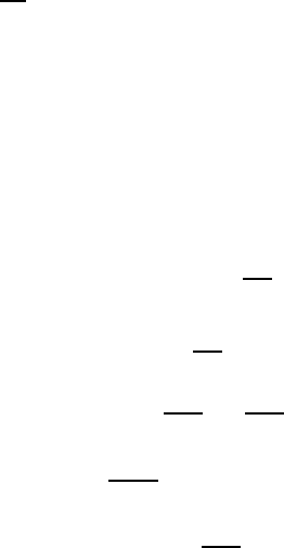
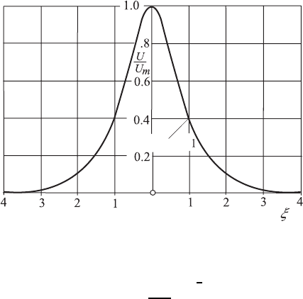
The velocity proﬁle that can be computed from the above equations is

shown in Fig. 16.11. The U

component of the velocity ﬁeld is computed at

the edge of the jet:

(ξ

∞

)=−0.55



ges

ρx



It is negative and this indicates that the free jet ﬂow continuously sucks in

ﬂuid from the outer ﬂow, so that the mass ﬂow of the free jet increases in the

ﬂow direction.

The mass ﬂow can be computed at each point x of the free jet:

˙m = ρ

+∞

−∞

dy, (16.113)

486 16 Flows of Large Reynolds Numbers

Velocity profile

for 2-dim . jet

−−−−

Fig. 16.11 Velocity proﬁle of the plane free jet ﬂow

˙m =3.3



ges

νx



. (16.114)

The ﬂuid input into the free jet ﬂow takes place due to the viscosity of the

ﬂuid, i.e. the entrainment is caused by the molecular momentum transport.

16.7 Plane, Two-Dimensional Wake Flow

Additional ﬂows that are important in practice and that can be treated with

the aid of the boundary-layer equations, are wake ﬂows showing the features

sketched in Fig. 16.11. This ﬁgure shows a plane, two-dimensional wake ﬂow

as occurs, e.g., behind a plane plate or a cylinder located with the main axis

perpendicular to the x–y plane. Such ﬂows are characterized by a momentum

deﬁcit, which corresponds in its integral properties to the ﬂow resistance force

of the plate or cylinder around which a ﬂow passes. This can be computed

by employing the integral form of the momentum equation:

=2ρB

∞

− U

)dy, (16.115)

where U

(y) represents the velocity proﬁle of the wake ﬂow existing at a

certain x-position, B is the width of the plate in z-direction, and U

∞

corre-

sponds to the main ﬂow in the x-direction at y →∞. For the inﬁnitely thin

plane plate, one obtains the result

=2ρBU

∞

. (16.116)

For the cylinder one obtains

16.7 Plane, Two-Dimensional Wake Flow 487

Fig. 16.12 Wake ﬂow behind a body around which a ﬂow takes place

= c

∞

!d. (16.117)

Although the actual ﬂow structure near the plate or cylinder around which

the ﬂow passes can be complicated, the ﬂow in the downward ﬁeld proves to be

of the kind that becomes independent of the body which generated the wake

ﬂow. In the downstream region, the ﬂow has a boundary-layer ﬂow structure,

as the ﬂuid ﬂow in the x-direction of the wake takes place convectively and

the transverse distribution is established by diﬀusion.

For the treatment of the wake ﬂow, sketched in Fig. 16.12, the velocity

diﬀerence can be expressed as

u(x

)=U

∞

− U

) (16.118)

and it is this diﬀerence that is introduced into the boundary-layer equations.

When considering that the pressure in the entire ﬂow region is constant and

that moreover, because u(x

) << U

∞

holds, one can write

∞

− u)

∂

∂x

∞

− u) ≈ U

∞

∂u

∂x

= ν

∂

∂x

(16.119)

and, hence, one obtains the diﬀerential equation that is to be solved for the

wake ﬂow. The boundary conditions can be stated as

=0:

∂u

∂x

=0 and x

→∞: u =0. (16.120)

Similarly to the earlier ansatzes, the following relationships are introduced.

η = x

∞

νx

and u = U

∞





−1/2

f (η) (16.121)

and (16.121) introduced into (16.115) yields

= ρBU

∞



ν!

∞



1/2

+∞

−∞

f(η)dη. (16.122)

488 16 Flows of Large Reynolds Numbers

On introducing (16.121) into (16.119), one obtains the ordinary diﬀerential

equation to be solved for wake ﬂows:



ηf



f = 0 (16.123)

with the boundary conditions:

η =0:f



(η)=0 and η →∞: f (η) → 0. (16.124)

Equation (16.123) can be rewritten and integrated:

dη



ηf



=0,

dη



dη

ηf



= 0 (16.125)

so that following ﬁnal relationship holds:

dη

ηf = C ; C =0, since η =0

dη

=0. (16.126)

In this way, the solution for f(η) is obtained as an exponential function of

f(η)=exp



−



. (16.127)

With this, the following can be computed from (16.122):

= ρBU

∞



ν!

∞



1/2

+∞

−∞

exp



−



dη. (16.128)

For the ﬂat plate the value of K

can be computed by integration along both

plate sides:

=1.328BρU

∞

ν!

∞

(16.129)

so that for C in (16.128) one can deduce C =0.664/

√

π. Hence, one obtains

for the velocity proﬁle of the wake ﬂow behind a ﬂat plate:

)=U

∞

− U

∞

0.664

√





−1/2

exp



−

∞



. (16.130)

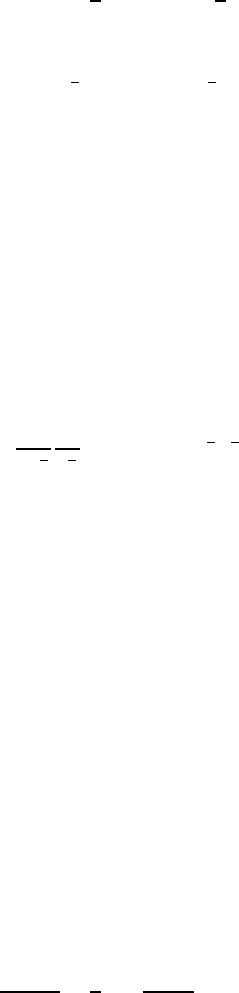
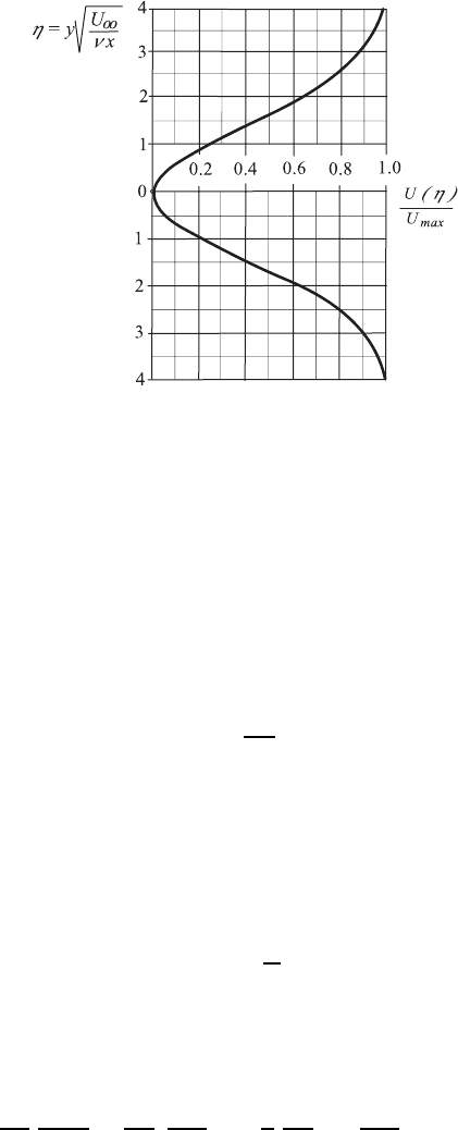
This somewhat asymptotic solution is given in Fig. 16.13, namely for the

diﬀerence velocity u(x

) ; U(η), normalized with the local maximum of

the “deﬁcit velocity”:

max

= U

∞

0.664

√





−1/2

, (16.131)

i.e. U(η)/U

max

is plotted in Fig. 16.13.

16.8 Converging Channel Flow 489

−

Fig. 16.13 Solution for the normalized wake ﬂow behind a plate

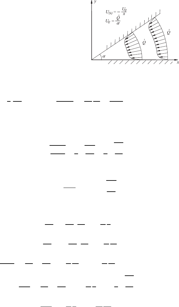
16.8 Converging Channel Flow

The boundary-layer ﬂows considered above, were all characterized by an outer

ﬂow with constant velocity. They thus represent the easiest ﬂows which can

be solved with aid of the boundary-layer equations.

Based on the solution procedure derived by Blasius, in this section the

boundary layer of a ﬂow will be considered, whose imposed ﬂow is given by

the following velocity distribution:

∞

(x)=−

= U(x), (16.132)

where U

Q/x, i.e. is the velocity existing at x = 1. When considering that

the velocity distribution corresponds to that of a sink ﬂow in a convergent

channel with an aperture angle α between the plane walls, then the volume

ﬂow rate ﬂowing through the region α

Q = αxhU

is given for h =1by

αU

, i.e. the following holds:

. (16.133)

Because of the above-suggested velocity distribution of the ﬂow, outside the

developing boundary layers, a pressure gradient results in the stationary

boundary-layer equation:

∂Ψ

∂y

∂

∂x∂y

−

∂Ψ

∂x

∂

∂y

= −

+ ν

∂

∂y

. (16.134)

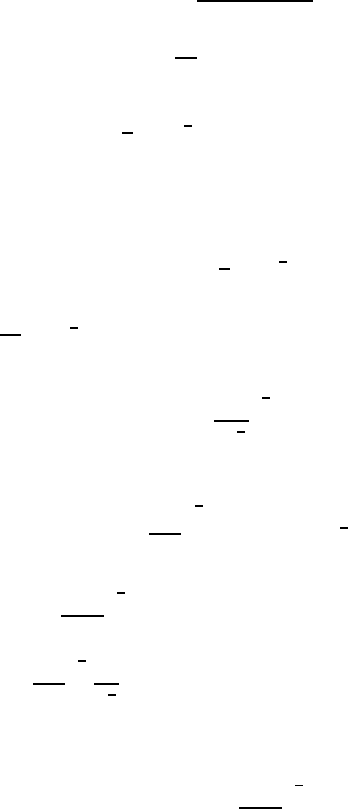
490 16 Flows of Large Reynolds Numbers

Fig. 16.14 Diagram to explain boundary-

layer formation in a converging two-

dimensional channel ﬂow

The resulting pressure gradient can be computed as:

= −U

∞

(x)

dU(x)

αx

. (16.135)

In order to obtain the sought similarity solution for the boundary layer

which forms at the walls of a converging channel ﬂow (Fig. 16.14), the

following similarity variable is introduced:

η = y

−U

∞

xν

αν

. (16.136)

For the stream function of the ﬂow we introduce

Ψ(x, y)=−



νU

f(η)=−

Qν

f(η) (16.137)

so that for the diﬀerent terms in (16.38) the following relationships can be

derived:

∂Ψ

∂y

∂Ψ

∂η

∂y

= −



(η), (16.138)

= −

∂Ψ

∂x

= −

∂Ψ

∂η

∂x

= −



(η), (16.139)

∂

∂x∂y

∂

∂x



∂Ψ

∂y





(η)+



(η), (16.140)

∂

∂y

∂

∂y



∂Ψ

∂y



= −



(η)

αν

, (16.141)

∂

∂y

= −



(η)

αν

. (16.142)

On inserting (16.134) and also (16.136)–(16.140) in the boundary-layer equa-

tion (16.132), one obtains the following diﬀerential equation for f (η); only

16.8 Converging Channel Flow 491

a few terms remain, since the products of the mixed derivatives f





cancel

out:



− (f



)

+ 1 = 0 (16.143)

with the boundary conditions at η =0,f



= 0 and for η →∞,f



=1and



=0.

The integration of the above diﬀerential equation becomes analytically

possible with the ansatz

F (η)=f



(η) (16.144)

so that (16.143) can be written as



= F

− 1 with F (0) = 0 and F (∞)=1. (16.145)

On multiplying both sides with the ﬁrst derivative F



(η), it is possible, by

partial integration, to obtain the following solution:



)

−

(F − 1)

(F +2)=C, (16.146)

where C is the integration constant, which, because F → 1andF



→ 0as

η →∞, adopts the value C = 0. Hence, from (16.146) it follows that



dη

(F − 1)

(F + 2) (16.147)

or rewritten:

dη =



(F − 1)

(F +2)

. (16.148)

Hence, the following equation holds:

η =



(F − 1) (F +2)

. (16.149)

The integral can be given in a closed form:

η =

tanh

−1

√

2+F

√

− tanh

−1

. (16.150)

Solved in terms of F =

= f



(η):



(η)=

=3tanh



√

+ln



√





− 2 (16.151)