Durst F. Fluid Mechanics: An Introduction to the Theory of Fluid Flows

Подождите немного. Документ загружается.

12.5 Flow with Heat Transfer (Pipe Flow) 349

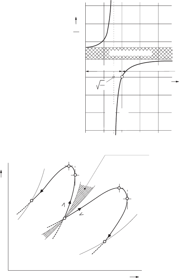
Fig. 12.11 Change of state in the T–s diagram for pipe ﬂows with heat supply

that (12.89) holds not only for ﬂows of ideal gases, generally treated in gas

dynamics, but also for the ﬂows of real gases.

In conclusion, it can be remarked that the relationships for

(12.74),

dρ

(12.75),

(12.76),

(12.76) and

dMa

(12.78) for Ma =1losetheir

validity if (dq) = 0. In order to accelerate a subsonic ﬂow to supersonic ﬂow

speeds through heat supply, the heat supply has to be stopped once Ma =1

is reached. After that, it is necessary to cool the ﬂow in order to obtain a

further velocity increase.

Extended considerations show that the heat supply in the subsonic region

leads to accelerating the ﬂow and in the supersonic region to decelerating the

ﬂow. For pipe ﬂows with a radius R = constant, a subsonic ﬂow cannot be

turned into a supersonic ﬂow with constant heat supply.

By considering the course of the eﬀective heat capacity of the pipe ﬂow,

the behaviour shown in Fig. 12.12 results:

(Ma

− 1)

(Ma

− 1/κ)

. (12.90)

For 0 ≤ Ma <



1/κ and 1 ≤ Ma < ∞ the heat capacity is positive and in

the range



1/κ < Ma < 1 a negative heat capacity results. At Ma =



1/κ

the local ﬂow velocity has the value of the isothermal sound velocity.

According to (12.88) for the eﬀective heat capacity c

in heated and

cooled pipe ﬂows, the thermodynamic state developes as shown in Fig. 12.13.

350 12 Introduction to Gas Dynamics

Fig. 12.12 Behavior of the eﬀec-

tive heat capacity of a gas with heat

supply in a pipe ﬂow

Forbidden region

Subsonic

Supersonic

Isothermal

sound velocity

Isentropic

sound velocity

const

′

const.

const

From C´ to B´ cooling

on subsonic

Heating from A to C

From C to B cooling

M 1

M´ 1

Forbidden region

on subsonic

Fig. 12.13 Thermodynamic changes of state at subsonic and supersonic pipe ﬂows

accordingtoBoˇsnjakovi´c

Starting for subsonic ﬂow from state A, one reaches state C by heating

and subsequently state B by cooling, where a supersonic ﬂow is achieved. If,

on the other hand, state A is supersonic, heating would decelerate the ﬂow

towards C



and ﬁnally cooling would further decelerate to subsonic ﬂow B



12.6 Rayleigh and Fanno Relations 351

12.6 Rayleigh and Fanno Relations

The considerations in the preceding section concentrated on the investigation

of inﬁnitesimal changes of ﬂuid-mechanical and thermodynamic state quan-

tities in pipe ﬂows, i.e. on the changes in the case of an inﬁnitesimal heat

supply to the ﬂuid, with the assumption that no dissipative processes occur.

For the pressure and Mach number changes that occur, it was derived that:

−κMa

(1 − Ma

)

(dq)

and

dMa

(1 + κMa

)

(1 − Ma

)

(dq)

. (12.91)

From these, the following relationship between the relative changes of

pressure and Mach number for the pipe ﬂow is obtained:

= −

κMa

(1 + κMa

)

(dMa

)

. (12.92)

This diﬀerential equation can be integrated between two states 1 and 2,

yielding:

= −

κMa

(1 + κMa

)

dMa

; ln





=ln



1+κMa



(12.93)

and thus:

1+κ(Ma)

etc.. (12.94)

From (12.53), a thermodynamically achievable maximum pressure P

fol-

lows:

= P



κ − 1



(κ−1)

. (12.95)

With this relationship, also known as the Rayleigh ﬂow, the following case

can be computed:

)

(1 + κMa

)

(1 + κMa

)

(κ−1)

. (12.96)

Analogously for the temperature relationship T

, the following can be

derived:

(Ma)

1+κ(Ma)

, (12.97)

352 12 Introduction to Gas Dynamics

and for the corresponding relationship of the stagnation temperature ratio:

)

1+κMa

(κ−1)

. (12.98)

For the density and velocity relationship one can write:

1+κMa

. (12.99)

Finally, the following relationship can also be derived:

ds = c



1 − Ma

1+κ · Ma



d(Ma

)

(12.100)

in order to compute the entropy change of the ﬂowing gas in the pipe ﬂow

with heat supply, the following holds:

− s

κR

(κ − 1)



 

·ln

⎡

⎢

⎣

(Ma)

1+κ(Ma)

(κ+1)

⎤

⎥

⎦

. (12.101)

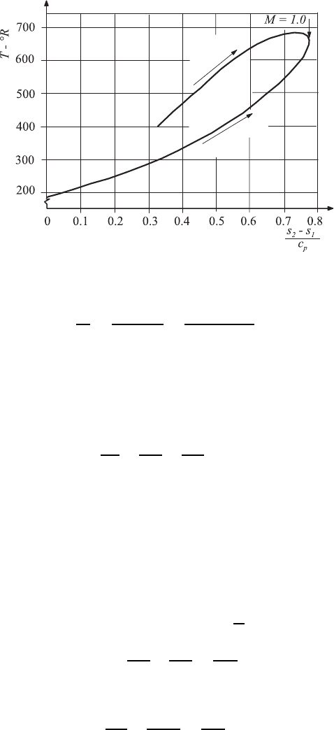
The above equations can now be employed to determine in a T −s diagram

the thermodynamically possible states with the Mach numbers as parameters,

e.g. for Rayleigh ﬂow. We start here from a state 1, for which T

and s

are

known, as well as U

and therefore also (Ma)

.Foreachvalue(Ma)

, T

can be computed and thus the Rayleigh curve, as shown in Fig. 12.14 can

be obtained. For the direct connection between s and T one obtains:

− s

=ln





κ+1

2κ

From Fig. 12.14, it can be seen that for the subsonic part of the Rayleigh

curve the temperature increases, together with an increase in the Mach num-

ber up to Ma =



1/κ. After that the temperature decreases until Ma =1.

On moving on the branch of the supersonic ﬂow, the Mach number decreases

with increasing entropy until Ma = 1 is achieved.

It is also usual in gas dynamics to employ values for (Ma)

=1,which

are usually designated with an asterisk (∗) as reference quantities for the

standardized representation of P , P

, T , T

and ρ. For such a representation

of the above results, the following holds:

∗

1+κ

1+κMa

;

∗

(1 + κ)

(1 + κMa

)

, (12.102)

12.6 Rayleigh and Fanno Relations 353

Supersonic

Heating

Subsonic

Fig. 12.14 Rayleigh curves on a T–s diagram

∗

)

1+κMa

(1 + κ)Ma

. (12.103)

A generalization of the considerations above for ﬂows in pipes with change

in cross-section, which are furthermore exposed to externally imposed forces,

leads to the relationships below for the ﬂuid mechanical and thermodynamic

changes of state caused in compressible ﬂows.

Continuity equation:

dρ

=0. (12.104)

Momentum equation:

ρU dU = −dP +dΠ, (12.105)

where dΠ is an externally applied pressure gradient which can be forced on

the ﬂow by a compressor. The energy equation can be stated for the extended

considerations as follows:

dT + U dU

=dq. (12.106)

By division by P and after introduction of c

= κ

, the momentum (12.105)

can be written as

κMa

dΠ

. (12.107)

For the energy equation, the following rearrangements of terms are

possible:

U dU

, (12.108)

354 12 Introduction to Gas Dynamics

or rewritten:

+(κ − 1)Ma

. (12.109)

Finally, the state equation for ideal gases is employed for the considerations

to be carried out:

= RT ;

−

dρ

−

=0. (12.110)

The above set of equations can now be employed to express the quantities

dU/U, dρ/ρ, dT/T, etc. as a function of the local Mach number and the

local relative area change (dF/F), the heat supplied (dq/h) and the applied

external forces (dΠ/P ):

(Ma

− 1)



dΠ

−



, (12.111)

= −

κMa

(Ma

− 1)

−

1+(κ − 1)Ma

(Ma

− 1)

dΠ

κMa

(Ma

− 1)

, (12.112)

= −

(κ − 1)Ma

(Ma

− 1)

−

(κ − 1)Ma

(Ma

− 1)

dΠ

(κMa

− 1)

(Ma

− 1)

. (12.113)

From the above general equations, the preceding derivations, that are referred

solely to the area changes (see Chap. 9), can now be derived for dΠ/P =0

and dq/h =0.Furthermore,oneobtainsfor dF/F =0and dΠ/P =0the

relationships derived at the beginning of this chapter for heated pipes. When

one now sets dF/F =0anddq/h =0,oneobtains:

(Ma

− 1)

dΠ

;

= −

1+(κ − 1)Ma

(Ma

− 1)

dΠ

, (12.114)

and ﬁnally also:

= −

(κ − 1)Ma

(Ma

− 1)

dΠ

. (12.115)

On considering now for a viscous ﬂow the molecular momentum transport

as an external action of forces (dΠ

/P ) < 0, one realizes that the following

temperature changes are connected with it:





> 0forMa < 1, (12.116)





< 0forMa > 1. (12.117)

Analogous to the considerations that were based on (12.91) and (12.92),

all derivations that lead to the relationships for the Rayleigh ﬂow, i.e. for the

12.7 Normal Compression Shock (Rankine–Hugoniot Equation) 355

ﬂow through pipes having constant cross-sections with heat supply, can now

be repeated for pipe ﬂow under the inﬂuence of friction without heat supply.

From the derivations, similar relationships result as for the Rayleigh ﬂow in

(12.94)–(12.102). From, this the “Fanno curve” in the T– s diagram results,

which indicates the possible states of the thermodynamic state that develop

in adiabatic pipe ﬂow with internal friction. The “Rayleigh curve” in the T–s

diagram, on the other hand, represents the thermodynamic change of state

which develops with heat supply in the case of friction-free ﬂow of an ideal

gas in a pipe. With this the Fanno curve indicates the inﬂuence of friction

in a pipe ﬂow with constant cross-section, whereas the Rayleigh curve shows

the inﬂuence of the heat supply.

12.7 Normal Compression Shock

(Rankine–Hugoniot Equation)

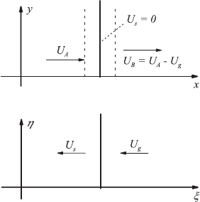
In Sect. 12.3, the formation of compression shocks was explained as a

phenomenon of wave motions with a state-dependent wave velocity. The

discontinuity surface formed in this way shows a thickness which can be

considered to be of the order of magnitude of the free path length of the

molecules of an ideal gas. It is thus possible to describe, within the assump-

tions chosen in this book, the compression shock shown in Fig. 12.15 in a

medium at rest by the ﬂuid mechanical and thermodynamic state quantities

before and after the compression shock. As before, the analysis may be sim-

pliﬁed by considering a stationary problem, i.e. assuming that the shock is at

rest. The ﬂow velocity and the variables describing the thermodynamic state

upstream of the shock are denoted by P

, ρ

, T

, e

, s

and downstream by

, ρ

, T

, e

, s

. Thus the transformation is U

= U

and U

= U

−U

respectively.

Fig. 12.15 Plotted normal compression

shocks and selection of coordinate systems

356 12 Introduction to Gas Dynamics

The integral conservation laws formulated with these variables are

expressed as:

= ρ

− U

)=ρ

, (12.118)

+ P

= ρ

+ P

, (12.119)

or rewritten:

− U

)=P

− P

. (12.120)

Furthermore, the energy equation holds:

+ c

. (12.121)

The left-hand side of (12.121) can be described by the quantities P , ρ and U

of the mass conservation and momentum equations as one obtains:

+ c

Rρ

(κ − 1)

. (12.122)

From the momentum equation and the continuity equation, it follows that:

− U

−

. (12.123)

Multiplication by U

+ U

yields:

− U



−



+ U

), (12.124)

− U



−



, (12.125)

or rewritten:

− U

=(P

− P

)





. (12.126)

From the energy equation it follows:

− U

2κ

κ − 1



−



. (12.127)

Equations (12.125) and (12.126) set equal yields:

− P

)





2κ

κ − 1



−



. (12.128)

From this, the following relationship is obtained:



−

(κ +1)

(κ − 1)



=1−

(κ +1)

(κ − 1)

. (12.129)

12.7 Normal Compression Shock (Rankine–Hugoniot Equation) 357

Hence one can write:

(κ +1)



− 1



1 −

(κ − 1)



− 1



and

(κ +1)

2κ



− 1



(κ − 1)

2κ



− 1



(12.130)

The above relations P

= f(ρ

/ρ

)or(ρ

/ρ

)=g(P

)areknown

as Rankine–Hugoniot equations. They state the pressure and density changes

through the normal compression shock. As the compression shock is linked

to a dissipation of mechanical energy into heat, the compression shock is a

non-isentropic process.

Derivations of somewhat diﬀerent nature, using the energy equation yield:

2κ

(κ − 1)

2κ

(κ − 1)

(12.131)

and

2κ

(κ − 1)

2κ

(κ − 1)

. (12.132)

From this, the following results:

− U

2κ

(κ − 1)



−





 

−U

2κ

(κ − 1)



−



(12.133)

− U

) −

2κ

(κ − 1)

− U

(κ − 1)

− U

, (12.134)

1 −

2κ

(κ − 1)

= −

(κ − 1)U

. (12.135)

From this, the Prandtl compression relationship can be computed:

(κ +1)

;(Ma)

A,H

(Ma)

B,H

(κ +1)

. (12.136)

From the energy equation:

+ c

= c

and

+ c

= c

. (12.137)

It then follows that:



(κ − 1) +

(Ma)



(κ − 1), (12.138)



(κ − 1) +

(Ma)



(κ − 1). (12.139)

358 12 Introduction to Gas Dynamics

Multiplying these two equations yields:



(κ − 1) +

(Ma)



(κ − 1) +

(Ma)



(κ − 1)

. (12.140)

With U

2κRT

(κ +1)

, the following equation results:



κ − 1



(Ma)



κ − 1



(Ma)





(κ +1)



. (12.141)

It is usual to express the state quantities, after the vertical compression shock,

scaled with the corresponding quantity before the shock, as a function of the

Mach number before the shock. These normalized quantities can be written

as follows:

2κ

(κ +1)

(Ma)

−

(κ − 1)

(κ +1)

;

=1+

2κ

κ +1

− 1

, (12.142)

(κ +1)(Ma)

(κ − 1)(Ma)

, (12.143)

(κ +1)

(Ma)

2κ(Ma)

− (κ − 1)

(κ − 1)(Ma)

(12.144)

Furthermore, it can be stated for the Mach number after the compression

shock:

(Ma)

(κ − 1)(Ma)

[(2(Ma)

− 1)κ +1]

, (12.145)

and for the pressure diﬀerence ∆p/p

as a measure for the strength of the

compression shock:

− P

)

2κ

(κ +1)

(Ma)

− 1

. (12.146)

For the change of entropy linked to the shock, one can compute:

− s

= c



2κ

κ +1

(Ma)

−

κ − 1

κ +1



(κ − 1)(Ma)

(κ +1)(Ma)





. (12.147)

The changes are shown in Fig. 12.17, where as the abscissa the Mach number

before the shock was chosen.