Du C., Xie L. Modeling and Control of Vibration in Mechanical Systems

Подождите немного. Документ загружается.

44 Modeling and Control of Vibration in Mechanical Systems

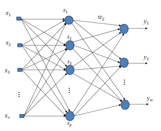
FIGURE 2.24

Three-layer RBF neural network.

Modeling of Disk Drive System and Its Vibration 45

weights. The output y

is given by

j=1

(kx −c

), i = 1, 2, ···, m, (2.46 )

or equivalently in a matrix form,

y(x) = W

s(x), (2.47)

where p is the number of nodes, x = [x

··· x

]

∈ R

is the network

input vector, k • k denotes the Euclidean norm, c

∈ R

is the center vector, and

= [w

]

The appro ximation of a general fun ct ion f(x) : R

→ R

can then be expressed

f(x) = W

s(x) + ε(x) (2.48)

where ε(x) ∈ R

is the reconstruction error vecto r.

Several functions such as Gaussian, Hardy’s multiquadric and inverse Hardy’s

multiquadric functions h ave been used as activation functions. They are separately

written as

(x) = exp[

−(x − c

)

(x − c

)

], (2.49)

(x) =

+ (x − c

)

(x − c

), (2.50)

and

(x) =

+ (x − c

)

(x − c

)

. (2.51 )

For a mechanical system with dynamics given as a f unction of positi on, velocity

and acceleration, a dynamic neural network is needed in order to fully emulate the

dynamics. In a dynamic neural network, dynamic vari ables such as velocity and

acceleration are involved in the input x. In discrete-time neural networks, past inf or-

mation such as x(k − 1) and x(k − 2) is u sed as inp ut.

2.4.2.2 Disturbance modeling

In some mechanical motion systems, disturbances in frequency range lower than a

few hundred Hz are quite d ominant and they may be due to torque distur bances,

nonlinear or unknown vibration sources. Here we use d

to represent these dis-

turbances. This section aims to model the low-frequency disturbance d

with an

46 Modeling and Control of Vibration in Mechanical Systems

adaptive nonli near strategy based on the measured error signal e. In t he open-loop

without controller C(z),

e = −P (s) ·d

−d

+ n. (2.52)

The disturbance d

is modeled as

= f(Φ(e(k))), (2.53 )

where f(·) is an unknown function of the bounded vector-valued function Φ(e(k))

with

e(k) = [e(k) e(k − 1) ··· e(k − l)]

, (2.54 )

where l is to be determined. Thus (2.53) is dependent on some time history of the

measured sign al e.

For brevity, f(Φ(e(k))) is denoted as f(Φ

). As stated i n the previous section,

the unknown fu nction f can be app roximated usin g neural networks. Here we se-

lect a Gaussian RBF based neural n et w ork. The Gaussian RBF network has some

attractive properties and thus has been widely used in nonli near control and signal

approximation. The properties are, (1) it is bounded and strictly positive, and (2)

it possesses a localized respon se. Based on the Gaussian RBF network, the l ow

frequency disturbances can be approximated as

= f(Φ

) = W

(k)s(Φ

) + ε, (2.55)

where ε is t he modeling error, s(Φ

) ∈ R

is a basis vector function with a suitable

number of n odes p. The radial basis fu nction s(Φ

) is wri tten as

(Φ

) = e

−

(e(k)−c

)

· e

−

(e(k)−e(k−1)−c

∆e

)

∆y

s(Φ

) = [s

(Φ

) s

(Φ

) ... s

(Φ

)]

, (2.56 )

where σ

and c

(σ

∆e

and c

∆e

) are the variance and center position of the mea-

surement e (velocity ˙e).

The weight vector W (k) in (2.55) can be calculated iteratively according to the

following weight update law:

W (k + 1) = (1 − δ)W (k) − Γs(Φ

)e(k) (2.57)

with the adaptation gain matrix Γ ∈ R

p×p

being diagonal and satisfying Γ > 0 and

the forgetting factor 1 > δ > 0 . The forgetting f actor δ is to ensure the bounded-

ness of W (k) when the system is subjected to boun ded disturbances. The speed of

learning rate is related to the chosen Γ matrix.

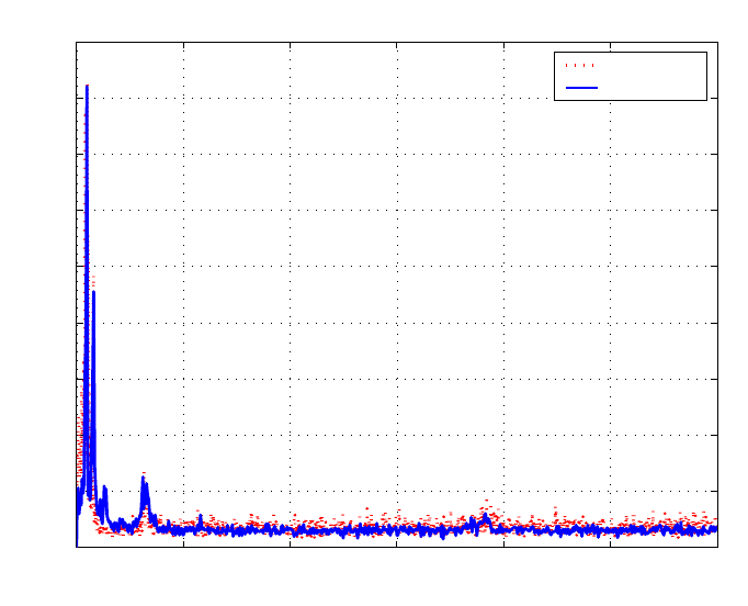
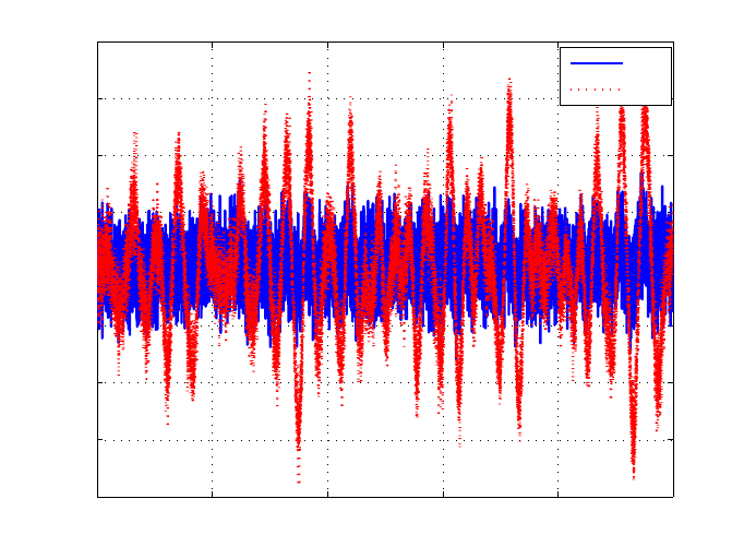
Next, the power spectrum in Figure 2.27 of a position error sign al e wil l be used to

verify the adaptive modeling scheme. It is noted that the contribution of disturbances

and noise to e is described as in (2.52).

Modeling of Disk Drive System and Its Vibration 47

A low frequency signal with the spectrum as in the low frequency range in Figure

2.27 is generated and injected as distur bance d

in Fi gure 2.21. The disturbance d

affects the error signal or the output e through the plant P (s), thus the nonlinear

model from e to

aims to generate a cancelation signal of the disturbance d

. Sin ce

the low frequency disturbances due to torque and bias are generally nonlinear, the

model from e to d

is chosen to be nonlinear.

The veriﬁcation is implemented with the sampling period T

= 1/4500 0sec. For

p = 1 with zero center positions c

and c

∆y

, after some trials, it was f ound that

when σ

= σ

∆y

= 10, δ = 0.5, and

Γ = T

· 10

·220, (2.58)

p = 1 , l = 1, (2.59)

the time trace

calculated from (2.55) gives the best approximati on of t he distur-

bance d

. The effect of different p and Γ on th e modeling accuracy will be evaluated

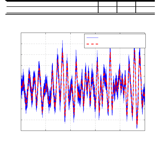
later. Figu re 2.25 shows the simulated time trace comparison of d

and

from the

nonlinear model (2.55). It is observed that the time trace fr om the model (2.55) can

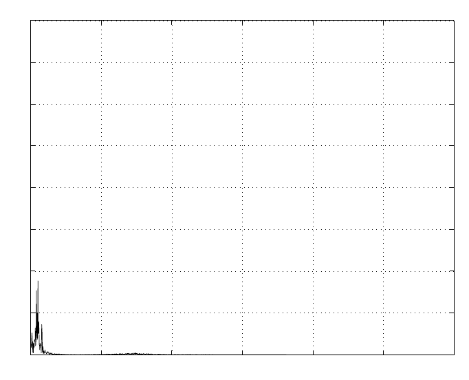
give a close tracking of the original one. The spectrum of

is seen in Figure 2.26.

Moreover, from the spectrum in Figure 2.27 with the component of disturbance

P (s) ·

removed and considering that noise n is a white noise, th e disturbance d

and the noise n are represented approximately by

= D

(s)w

, (2.60 )

(s) =

0.0019(s

+ 3329s + 1.695 × 1 0

)(s

+ 3340s + 5.61 × 10

)

+ 245s + 1.668 × 10

)(s

+ 477.5s + 5.70 1 × 10

)

and

ˆn = N (s)w

= 0 .005 w

. (2.61 )

The NRRO spectrum obtained by combining the n onlinear and linear models is

compared with t he measured one in Figu re 2.27 . It is found that the adaptive non lin-

ear modeling method can ind eed be used to model the distur bance d

that is dominant

in low f requency range.

Let the modeling error d

= d

−

. To evaluate the effects of different values of

p on the modeling error, two more cases with p = 5, 9 and the following parameters

for Γ are investigated.

Γ = T

· 10

· d iag{33, 66, 220, 66, 33}, p = 5; (2.62 )

Γ = T

· 10

· d iag{38.5, 88, 88, 38.5, 220, 38.5, 88, 88, 38.5},

p = 9 . (2.63 )

The σ value of t he modeling error e can be seen in Tabl e 2.1. With p = 1, 5, 9,

σ increases f rom 4.43 to 4.6 0, which means higher p may not give a better result

48 Modeling and Control of Vibration in Mechanical Systems

in this practical application. Compared with p, Γ inﬂuences the mod eling accuracy

more signiﬁcantly. For p = 1, with Γ being changed to 10% of the value in (2.58),

the σ value of the error e increases from 4.43 to 11. The time sequence comparison

of d

−

is shown in Figure 2.28, where the difference is clearly seen. The other

two cases are similar.

2.5 Conclusion

In this chapter the models of a VCM actuator and a PZT microactuator have been

derived on the basis of their physical operations. The models have been veriﬁed

with the measured frequency responses from voltage input to displacement output.

To have a complete model of an actuation system, this chapter has also addressed

the modeling of un certain ties in high frequency and nonlin earities such as actuator

pivot friction. A Prandtl operator based model has been used to model the friction

nonlinearity, and the optimal model parameters have been obtained by minimizing

the energy gain between the actuator position and the modeling error. It turns out that

the derived model matches well the measured model not only in the time domain, but

also in the frequency domain.

The developed vib ration and noise modeling approaches are based on the error

signal power spectrum of the closed-loop system. In particular, for low frequency

disturbance modeling, an adaptive nonlinear scheme with system measurement as

input has been applied to approximate the original disturbance for real-ti me com-

pensation.

Modeling of Disk Drive System and Its Vibration 49

TABLE 2.1

σ values of the modeling error (

− d

) for different p and Γ

p 1 5 9

σ values of (

−d

) for Γ and 0.1Γ.(×10

−4

) 4.43/11 4.55/11 4.60/10

0 0.05 0.1 0.15 0.2 0.25

−4

−3

−2

−1

x 10

−3

Time(sec)

Original disturbance and the modeled (µ m)

Original disturbance d

from nonlinear modeling

FIGURE 2.25

Original disturbance d

and the modeled

50 Modeling and Control of Vibration in Mechanical Systems

0 1000 2000 3000 4000 5000 6000

0.5

1.5

2.5

3.5

x 10

−3

Frequency(Hz)

NRRO magnitude(µm)

FIGURE 2.26

Power spectrum of

Modeling of Disk Drive System and Its Vibration 51

0 1000 2000 3000 4000 5000 6000

0.5

1.5

2.5

3.5

x 10

−3

Frequency(Hz)

NRRO magnitude(µm)

Modeled

Measured

FIGURE 2.27

NRRO power spectrum from measurement and disturbance models, i.e., e = −P (s)·

−

+ ˆn.

52 Modeling and Control of Vibration in Mechanical Systems

0 0.05 0.1 0.15 0.2 0.25

−4

−3

−2

−1

x 10

−3

Time(sec)

Modeling error (µm)

0.1Γ

FIGURE 2.28

Modeli ng error (d

−

) for different Γ with p = 1.

Modeling of Stewart P latform

3.1 Introduction

An adaptive control system i s able to adapt to th e changes of a physical system. In

order to obtain more accurate models for physical systems, adaptive identiﬁcation

algorithms can be used. Indeed, adaptive ﬁlterin g is often adopted in control and

signal processing ﬁelds, for the modeling of an unknown system.

In this chapter, the governing motion equation of a piezoelectric Stewart pl atform

will be obtained ﬁrst, fo llowed by th e derivation of a transfer function from the actua-

tor force to the sensor output based on frequency response data. An adaptive ﬁltering

approach will then be introduced and subsequently used to model the platf orm and

verify the t ransfer function obtained.

3.2 System description and governing equa tions

The stud y of active damping of ﬂexible structures has been induced b y the require-

ment of structural stability. Most solutions to the active damping problem rely on

the integration of smart actuators and sensors in the structure itself. Referring to the

discussion in Chapter 1, each leg of the hexapod Stewart platform consists of an am-

pliﬁed piezoelectric actuator, a force sensor and two ﬂexible joints. This piezoelec-

tric Stewart platform can be used as a precision pointing device, a vibration isolation

mount, or an active damping mou nt.

Shown in Figure 1.2 and Figure 1.3, the hexapod consists of two parallel plates

connected to each other by six active legs. The legs are mounted in such a way

to achieve the geometry of cubic conﬁguration . Each active leg consists of a force

sensor, an ampliﬁed piezoelectric actuator, and two ﬂexible joints.

Figur e 3.1 shows an equivalent system of each leg connecting two rigid bodies:

the disturbance source m and the sensitive payload M that are connected by a force

sensor and a piezoelectric actuator represented by its elongation δ and spring stiffness

k. The Laplace form of the governing equation of the motion in this system is