Du C., Xie L. Modeling and Control of Vibration in Mechanical Systems
Подождите немного. Документ загружается.

34 Modeling and Control of Vibration in Mechanical Systems
−4 −3 −2 −1 0 1 2 3 4
−2
−1.5
−1
−0.5
0
0.5
1
1.5
2
x 10
−3
Displacement (V, 0.5 µm/V)
Control signal u (V)
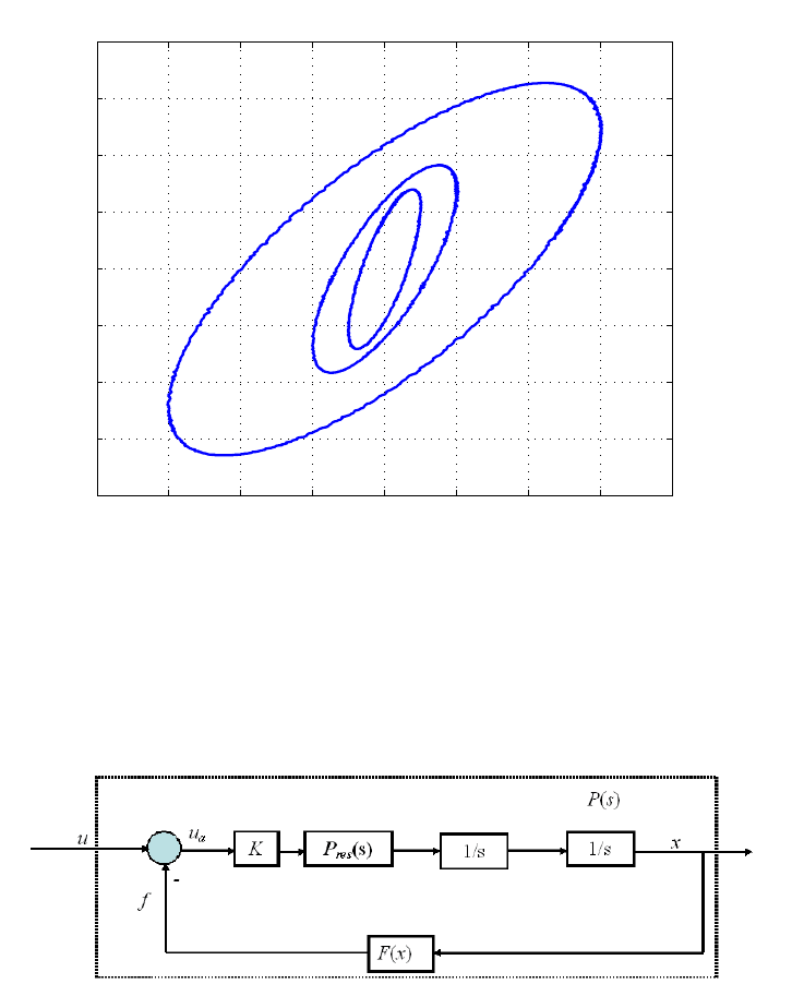
FIGURE 2.13
Control signal u versus displacement x.
FIGURE 2.14
VCM actuator modeling with friction nonlinearity model F (x).
Modeling of Disk Drive System and Its Vibration 35
In what follows, we shall find F (x) to model the relationship between f and x.
The above mentioned operator b ased method to approximate hysteresis will be ap-
plied to model the hysteresis of f and x as shown in Figure 2.6.
r
i
in (2.21 ) can be cho sen as the amplitud e of x. Since with the chosen peak-to-
peak values of x = 0.5 , 1 and 3V, the r
i
are respectively
r
1
= 0.25; r
2
= 0 .5; r
3
= 1 .5. (2.32 )
With m = 3, n = 3 and the initial valu es π
0
= 0, ξ
0
= 0, after 2000 iteratio ns, a
minimum error e is achieved and the optimal parameters are obtained as
a = 9.0024,
w
b1
= −1.5783, w
b2
= 0.1667, w
b3
= −0.0655,
w
c1
= −0.1431, w
c2
= −7.3341, w
c3
= 0.4403,
which gives the minimal kT
ex
k
∞
= 0.08.
With these parameters, f
e
= F (x(k)) can be calculated fro m (2.20). The time
traces of f
e
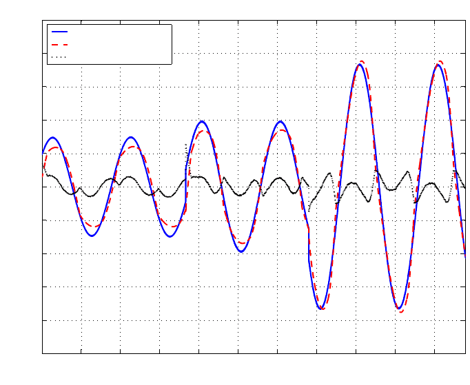
and f are compared in Figure 2.15. It is observed that the time trace
from the model (2.20) can closely track f, and the error f −f
e
is small. The modeled
hysteresis from x to f
e
is drawn and compared with the measured one i n Figure 2.6.
It is seen that the modeled hysteresis and the measured one are close to each other.
If th e creep term i n the model (2.20) is removed, i.e., w
cj
= 0, j = 1, ···, m, the
modeling accuracy decreases. Indeed, in this case, the minimal kT
ex
k
∞
= 0.1293 >
0.08.
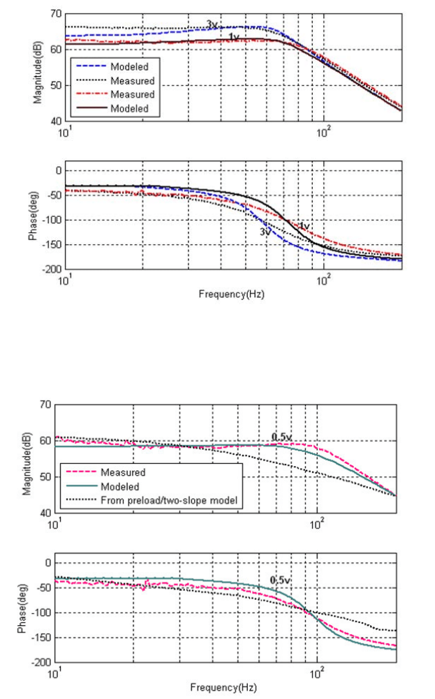
Figur es 2.16 and 2.17 show that the quality of the agreement in the frequency
domain between 70 Hz and 150 Hz decreases with lower excitation amplitude espe-
cially f or the 0.5V case.
Note that the operator model f
e
= F (x(k)) describes the hysteretic characteristics
in Figure 2.6 as a mapping between the actuator position x and the friction force
f. It turns out that the model makes it possible to approximate hysteretic transfer
characteristics withou t modeling the underlying physics. This is different from the
friction models such as the preload and two-slope model i n [40][42]. Compared to
the mod el in [40] [42], an advantage of our operato r based model is that the frequency
response of the actuator can also fit well to the measured one, as shown in Figures
2.16 and 2.17 .
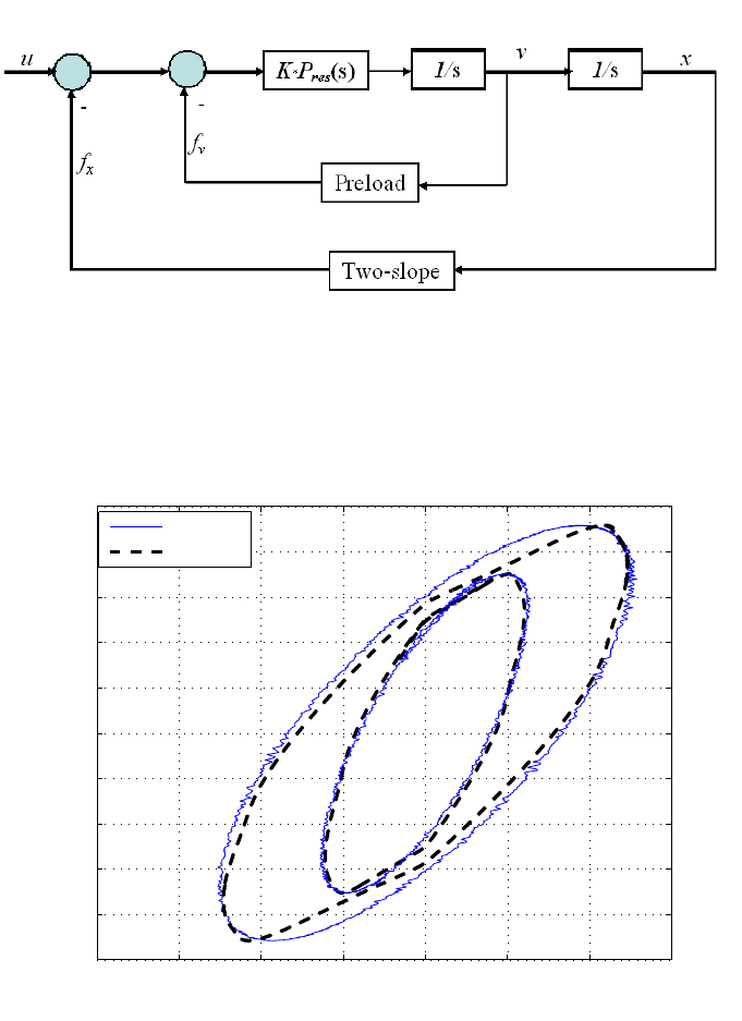
For comparison, we also apply the preload and two slope model [40] for the hys-
teresis, as shown in Fi gure 2.18. The preload model for velocity v and the two-slope
model for position x are given by
f
v
= k
v
v + k
s
sgn(v), (2.33)
and
f
x
=
k
a
x, |x| ≤ s
x
k
b
x + (k
a
−k
b
)s
x
, |x| > s
x
.
36 Modeling and Control of Vibration in Mechanical Systems
Using the data with the amplitude of x(t) of 0.25V, we obtain that
k
s
= 1.85e − 4, k
v
= 0.48, k
a
= 0.0145, k
b
= 0.0014, s
x
= 0.009.
Using this model, a comparison with the measured data in the time domain is
shown i n Figure 2.19 for the amplitude of x(t) of 0.5 and 1 V, respectively. It can
be o bserved that the plant input u versus position x fits reasonably well to the mea-
sured results in the time domain. However, in the frequency domain, the magnitude
response f or the case of the amplitude of x(t) of 0.5V, plotted as the dott ed curve in
Figur e 2.17 devi at es significantly from the measurement results.
0 0.05 0.1 0.15 0.2 0.25 0.3 0.35 0.4 0.45 0.5
−2.5
−2
−1.5
−1
−0.5
0
0.5
1
1.5
2
2.5
x 10
−3
Time(sec)
Friction and error
From measurement (f)
From modeling(f
e
)
Error (f−f
e
)
FIGURE 2.15
Measured and modeled friction and error.
Modeling of Disk Drive System and Its Vibration 37
FIGURE 2.16
Actuator frequency response for sinusoidal reference with amplitude of 1 and 3 V,
respectively.
FIGURE 2.17
Actuator f requency response for sinusoid al reference with amplitude of 0.5 V.
38 Modeling and Control of Vibration in Mechanical Systems
FIGURE 2.18
Preload and two-slope model for friction modeling.
−0.8 −0.6 −0.4 −0.2 0 0.2 0.4 0.6
−1
−0.8
−0.6
−0.4
−0.2
0
0.2
0.4
0.6
0.8
1
x 10
−3
Displacement (µm)
Input voltage u
Measured
Modeled
1V
0.5V
FIGURE 2.19
Plant input voltage u versus displacement x.
Modeling of Disk Drive System and Its Vibration 39
2.4 Vibration modeling
Vibration in disk drives causes the deviation of the R/W head po sitioning from the de-
sired track center. It is the combin at ion of the repeatable r unout which is synchronous
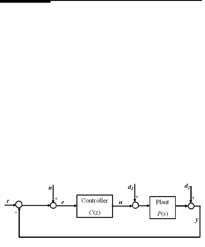
with the spin dle revolut ion and the nonrepeatable runout. Figure 2.20 shows a sim-
plified block-diagram of disk drive servo loop. y is the position of the R/W head and
e is the position error signal. The si gnal d
1
represents all the torque disturb ances
to the syst em. Such disturbances include any torque due to air-turbulence force to
the actuator, the suspension and the slider. The effects of the t orque disturbances are
dominant at frequencies that are r elat ively low when compared to the servo band-
width. The sign al d
2
represents d isturbances that are due to non-repeatabl e motions
of the disk and motor, suspension and slid er vibrations, which dir ectly add to the
relative p osition of the R/W head and the servo track. The noise si gnal n includes
media and head sensin g noises and also represents the effects of the PES demodu-
lation noise which includes actual electrical noise and A/D quantization noise. The
noise signal n is thus reasonably modeled as a broad-band white noise.
2.4.1 Spectrum-based vibration modeling
FIGURE 2.20
Closed-loop control system disturbances d
1
, d
2
and noise n.
Since a controlled closed-loop can provid e steady signals, the vibration source
analysis is based on the signal that is collected f rom the closed-loop system. From
Figur e 2.20 ,
e(k) = −P (z)S(z)d
1
(k) − S(z)d
2
(k) + S(z)n(k), (2.34)
40 Modeling and Control of Vibration in Mechanical Systems
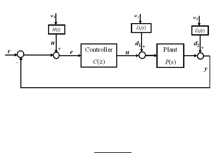
FIGURE 2.21
Closed-loop control system with di sturbance and noise models.
where P (z) is the transfer function of the discretized plant model P (s) and the sen-
sitivity function or error rejection function is given by
S(z) =
1
1 + P (z)C(z)
. (2. 35)
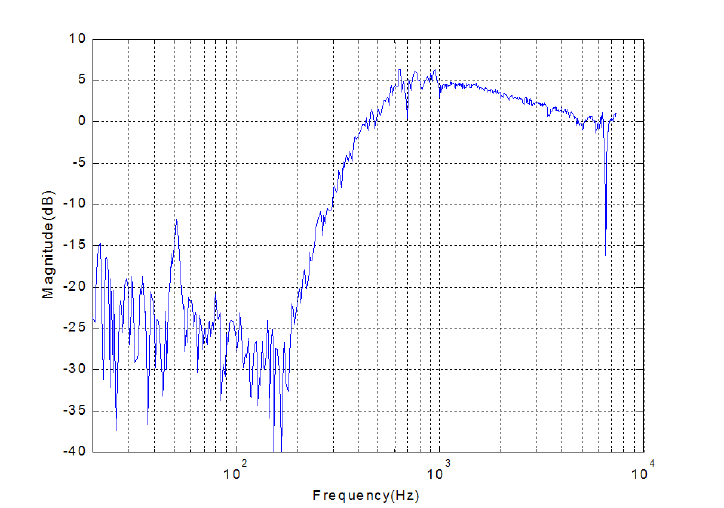
Figur e 2.22 shows the sensitivity function S(z) of a closed-loop control system.
Assume that d
1
, d
2
, and n are uncorrelated. The power sp ectrum denoted by S
e
of
the error signal e is given by
S
e
= |P (z)S(z)|
2
|d
1
(k)|
2
+ |S(z)|
2
|d
2
(k)|
2
+ |S(z)|
2
|n(k)|
2
. (2.36)
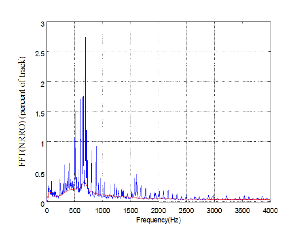
Figur e 2.23 shows the spectrum of NRRO component in the error signal e. Two
humps are obviously observed in the baseline curve. One is in t he fr equ ency range
lower than 100 Hz, th e other one is after 500 Hz. Considering (2.36) and Fig ure
2.22, the second hump is caused by S(z) through |S(z)|
2
|n(k)|
2
, and the first hump
is due to d
1
through P (z)S(z) with a hump in a lower frequency range. Hence the
disturbance and noise modeling can be carried out as foll ows.
In Fig ure 2.21, models D
1
(s), D
2
(s) and N(s) are used to describe d
1
(s), d
2
(s)
and n(s) respectively, and w
i
(i = 1, 2, 3) are independent white noises with
variance 1. Eq. (2.36) becomes
S
e
= |P (z)S(z)|
2
|D
1
(z)|
2
+ |S(z)|
2
|D
2
(z)|
2
+ |S(z)|
2
|N(z)|
2
, (2.37)
where D
1
(z), D
2
(z) and N (z) are the discrete forms of D
1
(s), D
2
(s) and N (s),
respectively. D
1
(z) and N (z) can be determined by fitting wei ghted versions of
P (z)S(z) and S(z) to the baseline curve of the spectrum and the spik es are consid-
ered as the effect of D
2
(z). Hence the steps to obtain D
1
, N and D
2
are
Modeling of Disk Drive System and Its Vibration 41
FIGURE 2.22
Sensitivity function S(z).
42 Modeling and Control of Vibration in Mechanical Systems
FIGURE 2.23
PES NRRO spectrum.
Step 1). Find S
b
(j),
S
b
(j) =
jq
min
i=1+(j−1)q
S
e
(i), j = 1, 2, ···, L/q, (2.38 )
where L is the length of S
e
and q is as small as possibl e.
Step 2). Compute D
1
(z),
|D
1
(z)|
2
= W
L
(z)S
b
/|P (z)S(z)|
2
, (2. 39)
where W
L
is a low-pass weighting function used to select S
b
in low frequency range.
Step 3). Compute N(z),
|N(z)|
2
= W
H
S
b
/|S(z)|
2
, (2.40)
where W
H
is the high-pass weighting function to select S
b
in h igh frequency range.
Step 4). Till now, the baseline curve S
b
can be fit wel l by the i dentified D
1
and N.
The remaining part o f the spectrum is then regarded as D
2
. Thus,
|D(z)|
2
= {S
e
− [|P (z)S(z)|
2
|D
1
(z)|
2
+ |S(z)|
2
|N(z)|
2
]}/|S(z)|
2
. (2.41 )

Modeling of Disk Drive System and Its Vibration 43
D
1
(s), D
2
(s) and N (s) are then obtained as follows from D
1
(z), D
2
(z) and
N(z) using the bilinear approxi mation method [81].
D
1
(s) =
1.3916 × 10
−5
(s + 575.8)(s + 575.6)(s
2
+ 0.04389s + 161.6)
(s
2
+ 315.5s + 8.17 8 × 10
4
)(s
2
+ 315.4s + 8.178 × 10
4
)
, (2.42)
D
2
(s) =
0.701588(s + 1 .271 ×10
4
)
2
(s
2
+ 6.125 × 10
−5
s + 4.373 ×10
8
)
(s + 708.4)
2
(s
2
+ 0.0001317 s + 4.376 × 10
8
)
,
(2.43 )
N(s) =
1.1695(s + 1.431 × 10
4
)(s + 766 .2)(s
2
+ 8609s + 4.672 × 1 0
7
)
(s + 4 603)(s + 1538)(s
2
+ 4451s + 1.507 × 10
7
)
. (2.44)
With t he disturbance and noise models, the feedback controller C(z) can be opti-
mized to minimize the erro r due to w = [w
1
w
2
w
3
]
T
by using the H
2
optimal control
method or other advanced cont rol methods.
2.4.2 Adaptive modeling of disturbance
2.4.2.1 Neural network approximation
A neural network usually consists of a large number of simpl e processing elements
called nodes. The nodes are interconnected by weighted links wit h weight param-
eters adjustable. The different arrangement of the nodes and the interconnections
defines various architectures of neural networks [73][74], which are suitable to dif-
ferent kinds of applicati ons. In control engineering, a multi-layer neural network
is usually used to generate the mapping from input to output since it can approxi-
mate any function under mild assumption with any desired accuracy. The function
approximation is defined as follows.
Definition 2.1 [75] If f(x) : R
n
→ R
m
is a continuous vector function defined
on a compact set Ω, and any y(W, x) : R
t
× R
n
→ R
m
is an approximatin g
function that depends continuously on W and x, then, the approximation problem is
to d et ermine the opti mal W denoted by W
⋆
, for some index d such that
d(y(W
⋆
, x), f(x)) ≤ ε, (2.45 )
for an acceptable small ε.
There are a number of neural networks studied for function approximation such as
multi-layer perceptron networks, radial basis function (RBF) networks, and higher
order neural networks. The RBF network is suitable for online non linear adaptive
modeling and control, because it is a linearly parameterized network , has spatiall y
localized learning capability and thus has better memory during learning, and ex-
hibits a fast initial rate of learning convergence.
The th ree-layer neural netw ork shown in Figure 2.24 is a RBF network, where
x ∈ R
n
, y ∈ R
m
, and s ∈ R
p
are respectively the input , the output, and the
activation function vectors, and w
ij
is the second to the third layer interconnection
