Du C., Xie L. Modeling and Control of Vibration in Mechanical Systems
Подождите немного. Документ загружается.

234 Modeling and Control of Vibratio n in Mechanical Systems
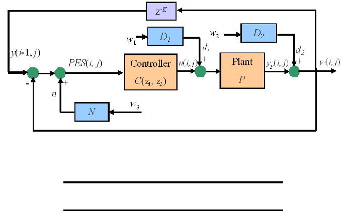
FIGURE 12.4
SSTW servo l oop modeling in two dimensions.
i = 0, 1, 2 , ···, L: the ith track.
j · T
s
: time with j = 0 , 1, 2, ···, K −1.
As shown in Figu re 12.4, y(i, j) i s the p osition of the write head at track i in the
radial dimension and ti me j · T
s
in the axial dimension and P ES(i, j) the po sition
error. y(i − 1, j) (i.e., y(j − K)) represents the track profile of the (i − 1)-th track.
Similarly, P ES(i − 1, j) represents the position error of the (i − 1)-th tr ack. The
read head follows the track y(i − 1, j) which is the reference input for the SSTW
servo system, i.e., one revolution of y(i, j) becomes the reference of the next written
track due to the action of self-servo track writi ng.
Based on Figure 12.4, we have
x
p
(i, j + 1) = A
p
x
p
(i, j) + B
p
(u(i, j) + d
1
(i, j)), (12.26)
y(i, j) = C
p
x
p
(i, j) + D
p
(u(i, j) + d
1
(i, j)) + d
2
(i, j), (12.27)
P ES(i, j) = y(i − 1, j) − y(i, j) + n(i, j). (12.28)
Denote x
p
, x
d
1
, x
d
2
and x
n
the corresponding state vectors of P (z), D
1
(z), D
2
(z)
and N(z), respectively. Let
x
h
(i + 1, j) = y(i, j), x
h
∈ R
n
h
, x
v
∈ R
n
v
,
x
v
(i, j + 1)
T
= [x
p
(i, j + 1)
T
x
d
1
(i, j + 1)
T
x
d
2
(i, j + 1)
T
x
n
(i, j + 1)
T
],
e(i, j) = P ES(i, j), w(i, j)
T
= [w
1
(i, j)
T
w
2
(i, j)
T
w
3
(i, j)
T
], (12.29)
it follows from (12.26)−(12.28 ) that
x
h
(i + 1, j)
x
v
(i, j + 1)
= A
x
h
(i, j)
x
v
(i, j)
+ B
1
w(i, j) + B
2
u(i, j), (12.30)
y(i, j) = C
1
x
h
(i, j)
x
v
(i, j)
+ D
11
w(i, j) + D
12
u(i, j), (12.31)

Two-D imensional H
2
Control for Error Minimization 235
e(i, j) = C
2
x
h
(i, j)
x
v
(i, j)
+ D
21
w(i, j) + D
22
u(i, j), (12.32)
where
A =
0 C
p
D
p
C
d
1
C
d
2
0
0 A
p
B
p
C
d
1
0 0
0 0 A
d
1
0 0
0 0 0 A
d
2
0
0 0 0 0 A
n
, B
1
=
D
p
D
d
1
D
d
2
0
B
p
D
d
1
0 0
B
d
1
0 0
0 B
d
2
0
0 0 B
n
, (12.33)
B
2
=
D
p
B
p
0
0
0
, C
1
=
0 C
p
D
p
C
d
1
C
d
2
0
, (12.34)
D
11
=
D
p
D
d
1
D
d
2
0
, D
12
= D
p
, (12.35)
C
2
=
1 − C
p
− D
p
C
d
1
− C
d
2
C
n
, (12.36 )
D
21
=
−D
p
D
d
1
−D
d
2
D
n
, D
22
= −D
p
. (12.37)
As such, the SSTW servo loop is modeled as the 2-D Roesser model (12.30)−(12.37)
[138] where disturbance and noise models are taken into consideration. The SSTW
error propagation problem can then be simplified as the stabilization problem of a
2-D system. Unlike 1-D feedback control plus feedforward compensation, it does
not need an add itional feedforward cont roller to prevent the error prop agation. In the
next section, feedforward compensation on the basis of 1-D feedback control will be
presented, followed by 2- D control in a later section.
12.5 Feedforward compensation method
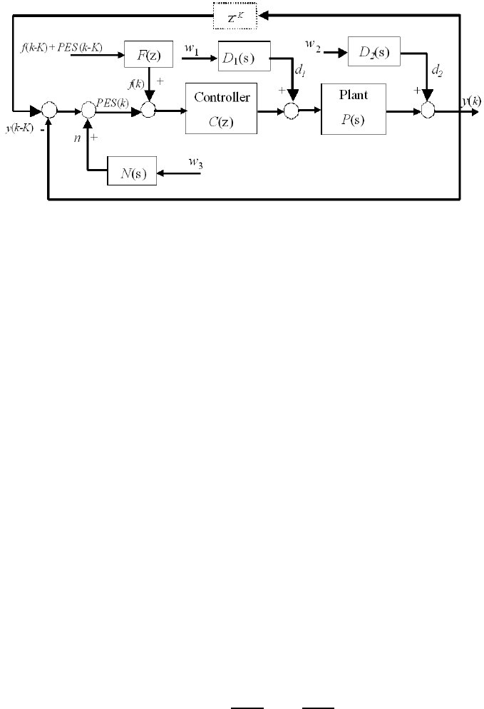
To contain the error propagation, it is easy to come up with the idea of injectin g a
correction signal f(k) to the PES by using the available signal P ES(k −K) through
a feedforward compensator F (z). Thus a feedforward (FF) compensatio n method is
used as shown in Figure 12.5.
During the servo writin g process, by tracking the previously written adjacent
tracks, adjusting servo reference and closing the existing VCM loop, the head can
be offset to a known radial position with reference to the adjacent tracks and gen-
erates radial information progressively to deploy servo pattern. The radial error in
one track is inevitably compounded to the following tracks and propagates accord-
ing to the closed-loop transfer fun ction from y(k − K) to y(k), as seen in (12.25).
The target of error propagation containment is thus to reject the written-in error due
to track no n-circularity recorded in propagated tracks so that the circular concentric
236 Modeling and Control of Vibratio n in Mechanical Systems
FIGURE 12.5
SSTW servo l oop.
tracks are achieved in every propagation trace. Obviously, when th ere is no hump in
the closed-loop transfer function T (z), the error propagation will be contained.
Next, we use three control schemes for the self-servo track writer: (1). PD con-
trol since it can produce a flat closed-loop response such that t he error propagation
is contained even without a feedforward compensation; (2). PID control pl us f eed-
forward compensation; (3). To minimize TMR or equivalently th e H
2
norm of the
transfer function from w = [w
1
w
2
w
3
]
T
to track profile y, the H
2
control tech-
nique is employed to design the feedback controller C(z) and then a feedforward
compensator F (z) is designed to contai n the error propagation.
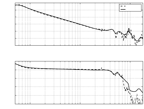
The frequ ency response of the VCM plant under consideration is shown in Figu re
12.6, and its transfer function P (s) is described by the following zeros, poles and
gain:
zeros = 10
4
×[3. 4558, − 0.6158 ± 8.7749j, 0.7540 ± 4.9697j,
−0.1960 ± 3.2614j, −0.9425 ± 1.6324j] , (12.38 )
poles = 10
5
×[−0.2513, − 0.3456, − 0.0726 ± 1.0342j, − 0. 0090 ± 0.5968j,
−0.0377 ± 0.3751j, − 0. 0283 ± 0.2813j,
−0.0011 ± 0.0036j], (12.3 9)
gain = 5.8987 × 10
12
. (12.40)
(1). PD feedback control
A typical form of PI D controllers is given by
C(z) = K
p
+ K
i
z
z − 1
+ K
d
z − 1
z
. (12.4 1)
Let K
i
= 0, a PD controller leading to a flat closed-loop transfer function can
be obtained by adjusting K
p
and K
d
. Denote the closed-loop transfer function as
Two-D imensional H
2
Control for Error Minimization 237
10
2
10
3
10
4
−60
−40
−20
0
20
40
60
Frequency(Hz)
Magnitude(dB)
Measured
Modeled
10
2
10
3
10
4
−1000
−800
−600
−400
−200
0
Phase(deg)
FIGURE 12.6
Frequency response of a VCM actuator.
238 Modeling and Control of Vibratio n in Mechanical Systems
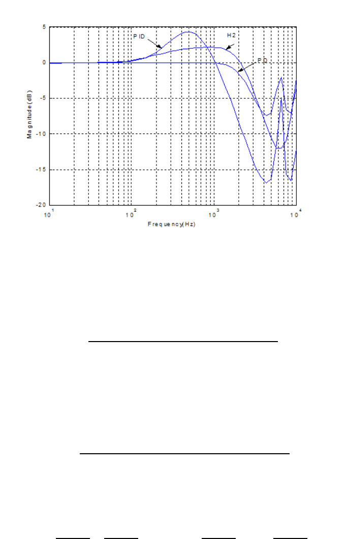
FIGURE 12.7
Frequency response of the closed-loop transfer function with the PD controller, PID
controller, and H
2
controller.
T
P D
(z). Figure 12.7 shows a flat magnitude response of T
P D
(z) resulting from the
PD controller given below. The sampling rate is 12.64 kHz.
C(z) =
4.79 × 10
−5
− 9.573 × 10
−5
+ 4.783 × 10
−5
z
2
− z
. (12.42)
Theoretically the error propagation would di sappear as kT
P D
k
∞
≤ 1. However,
the PD control is not able to deal with bias force due to lack of integrator. Simulation
shows that the prop agation stops after several tracks when a small bias force of 0.001
is added. Therefore, PD control is not practically applicable.
(2). PID feedback control pl us feedforward compensat ion
The closed-loop transfer function with the PID controller
C(z) =
2.435 × 10
−5
z
2
−4.406 × 10
−5
z + 1.999 × 10
−5
z
2
−1.209 + 0.24
(12.4 3)
has a region greater than 0 dB as seen in Figure 12.7. As mentioned earlier, this will
cause the error propagation problem. Thus a feedforward compensator F (z) will be
designed to contain the error propagation. According to Figure 12.5,
y(k) =
P C
1 + P C
+
F
1 + P C
y(k − K) +
P
1 + P C
d
1
(k) +
1
1 + P C
d
2
(k)
Two-D imensional H
2
Control for Error Minimization 239
+
P C
1 + P C
n(k) −
P F
1 + P C
d
1
(k − K) −
F
1 + P C
d
2
(k − K), (12.44)
which means that if the feedforward compensator F (z) is desig ned such th at the
magnitude of the transfer function
Φ =
P C
1 + P C
+
F
1 + P C
(12.4 5)
is less than one, i.e., kΦk
∞
< 1, the error propagation can be contained. It is
straightforward from (12.45) th at
F (z) = Φ(z)(1 + P (z)C(z)) − P (z)C(z). (12.46)
When Φ is selected as the closed-loop transfer function with the previous PD con-
trol, a 7
th
order F (z) is obtained from (12.46) after order reduction. The desig ned
F (z) can prevent the error propagation when the PID feedback control is applied in
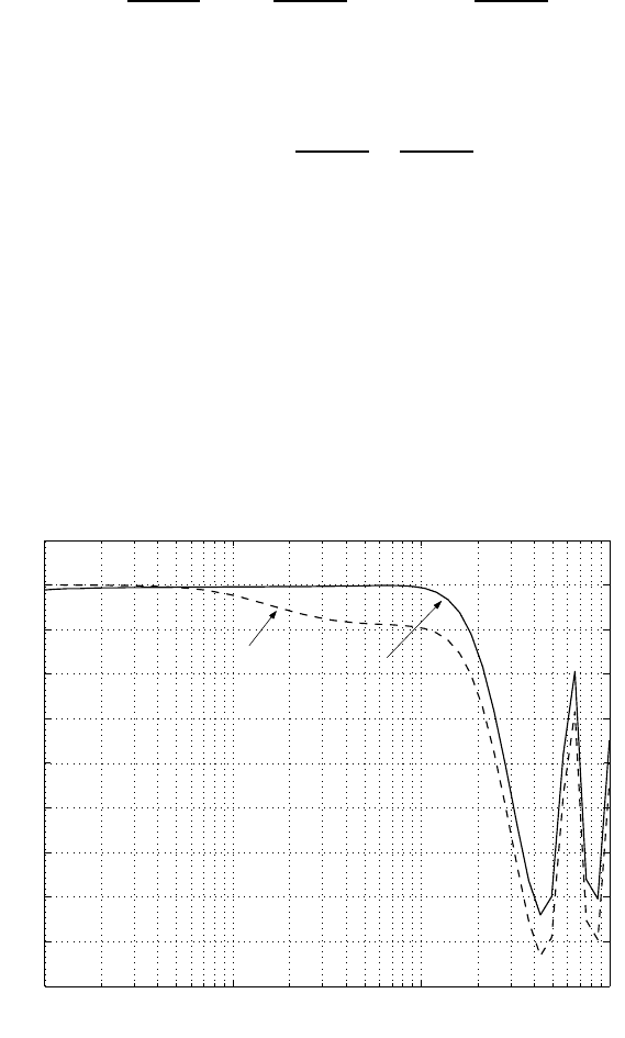
the servo l oop since kΦk
∞
< 1 with the designed F (z), as observed in Figur e 12.8.
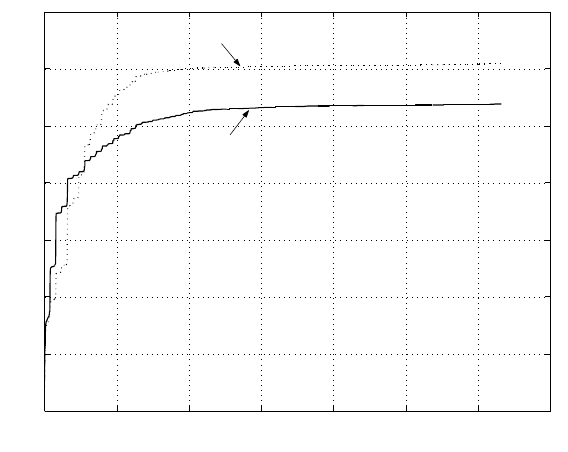
Figur e 12 .9 shows the 3σ value of the PES versus frequency wit h error propagation
containment.
10
1
10
2
10
3
10
4
−9
−8
−7
−6
−5
−4
−3
−2
−1
0
1
Frequency(Hz)
Magnitude(dB)
FF with H2
FF with PID
FIGURE 12.8
|Φ| versus frequency.
240 Modeling and Control of Vibratio n in Mechanical Systems
0 1000 2000 3000 4000 5000 6000 7000
2
4
6
8
10
12
14
Frequency(Hz)
3σ (percent of track)
PID
H2
FIGURE 12.9
3σ of PES NRRO.
(3). H
2
feedback control plus feedforward compensation
With the identified disturbance models in Chapter 2, the augmented system for the
optimal H
2
control design is described as follows.
x(k + 1) = Ax(k) + B
1
w(k) + B
2
u(k), (12.47 )
P ES(k) = C
1
x(k) + D
11
w(k), (12.4 8)
z(k) = C
2
x(k) + D
21
w(k) + D
22
u(k), (12.49)
where
A =
A
p
B
p
C
d
1
0 0
0 A
d
1
0 0
0 0 A
d
2
0
0 0 0 A
n
, B
1
=
B
p
D
d
1
0 0
B
d
1
0 0
0 B
d
2
0
0 0 B
n
, B
2
=
B
p
0
0
0
,(12.50)
C
1
=
C
p
0 C
d
2
C
n
, D
11
=
0 D
d
2
D
n
, (12.5 1)
C
2
=
C
p
0 C
d
2
0
, D
21
= 0, D
22
= 0, (12.5 2)
x is the combined state vari ables from the VCM actuator model P (z), the input dis-
turbance model D
1
(z), the output disturbance model D
2
(z), and the measurement
noise model N (z). (A
p
, B
p
, C
p
, D
p
), (A
d
1
, B
d
1
, C
d
1
, D
d
1
), (A
d
2
, B
d
2
, C
d
2
, D
d
2
),
and (A
n
, B
n
, C
n
, D
n
) are r espectively t he state-space models of P (z), D
1
(z),
D
2
(z) and N(z). P ES is the measured position error signal and z stands for y in
Figur e 12.5. The H
2
control problem can be solved using the method in Chapter 5.
Two-D imensional H
2
Control for Error Minimization 241
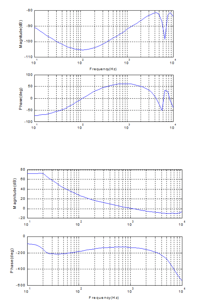
FIGURE 12.10
Frequency response of the H
2
controller.
FIGURE 12.11
Frequency response of the open-loop system with the H
2
controller.
242 Modeling and Control of Vibratio n in Mechanical Systems
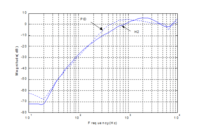
FIGURE 12.12
Comparison of sensitivity functions.
Figur es 12.10 and 12.11 show the frequency responses of the designed H
2
feed-
back controller and the compensated open-loop system wit h bandwidth of 1.07 kHz,
gain margin 7.3 dB, and phase margin 45.9 deg. Figure 12.12 shows the comparison
of error rejection functions with the PID control and the H
2
control, wh ere we can
see that the H
2
control outperforms the PID con trol in error rejection.
The frequency response of the closed-loop transfer function with the H
2
control
is shown in Figure 12.7, which impli es that a feedforward compensator is needed to
contain the error propagation when the servo lo op uses the H
2
feedback controller.
For the design of the feedforward compensator F (z), the selected Φ depends on the
feedback controller and it is found t hat lower Φ may not give a better error propaga-
tion contain ment. When Φ = 0.9T
P D
, a satisfactory error propagation containment
is guaranteed w hen the H
2
feedback control is appli ed in the SSTW servo lo op. A
6
th
order F (z) is t hus obtained after model reduction. The resultant |Φ| with the
designed F (z) is shown in Figure 12.8, and it is seen that |Φ| < 1. Figure 12.13
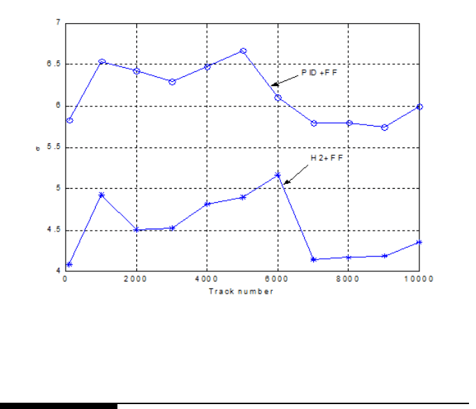
shows the σ value comparison of PES at d ifferent tracks with error propagation con-
tainment. It can be observed that PES σ is up and down as track propagation is going
on. Compared with that of the PID control, the σ of PES versus track number is
improved by around 27% when the H
2
control i s employed i n the SSTW servo loop.
Two-D imensional H
2
Control for Error Minimization 243
FIGURE 12.13
σ value of PES NRRO versus track number.
12.6 2 -D control formulation for SSTW
With the 2-D model (12.30)−(12.37), the SSTW error propagation problem is sim-
plified as the stabilization probl em of a 2 -D system. That is to design a dynamic out-
put feedback cont roller of the form in (12.9)−(12.10) for the model (12.30)−(12.32)
with w(i, j) = 0 such that the resulting closed-loop system is asymptotically sta-
ble. Unlike the design of 1-D feedback plus feedforward compensation previously, it
does not need an additional feedforward controll er to prevent the error propagation.
It is not difficult to see from (12.9)−(12.10) that (A
c2
, B
c2
, C
c
, D
c
) is acting
along the time direction only, and thus actually it works like the 1-D feedback con -
troller that we are concerned with conventionally.
The 2-D controller (12.21)−(12.22) can be written equivalently to the form (12.9)-
(12.10). Let
A
c1
=
I
n
h
0
0 0
A
c
, A
c2
=
0 0
0 I
n
v
A
c
, (12.53)
B
c1
=
I
n
h
0
0 0
B
c
, B
c2
=
0 0
0 I
n
v
B
c
. (12.5 4)
The performance of (A
c2
, B
c2
, C
c
, D
c
) can thus be evalu at ed as a normal 1-D
