Drake G.W.F. (editor) Handbook of Atomic, Molecular, and Optical Physics

Подождите немного. Документ загружается.

58 Part A Mathematical Methods

coupling symbol. Together these ranges enumerate ex-

actly the multiplicity n

of H

occurring in the reduction

of the multiple Kronecker product.

Uniqueness of state vectors:

| ( j

···j

)

···k

n−2

) jm









···j

···m







,... ,k

n−2

)

× |j

⊗···⊗|j

 .

In the C-coefﬁcient, the



are paired in the binary

bracketing. Each such C-coefﬁcient is a summation over

a unique product of n−1 SU(2) WCG-coefﬁcients.

Equivalent basis vectors:

| ( j

···j

)

···k

n−2

) jm

=±|( j



···j



)

···k

n−2

) jm ,

if and only if ( j

···j

)

∼ ( j



···j



)

.In-

equivalent basis vector are orthonormal in all quantum

numbers labeling the state vector.

Recoupling coefﬁcients:

A recoupling coefﬁcient is a transformation coefﬁ-

cient

( j

)



(l) jm

( j

)

(k) jm

relating any two orthonormal bases of the space H

⊗

···⊗H

, say, the one deﬁned by (2.103, 2.104),

and (2.110) for a prescribed coupling scheme corre-

sponding to a bracketing B, and a second one, again

deﬁned by these relations but for a different coupling

scheme corresponding to a bracketing B



. For example,

for n = 3, there are 3 inequivalent coupling symbols

and



= 3 recoupling coefﬁcients; for n = 4, there

are 15 inequivalent coupling symbols and



= 105

recoupling coefﬁcients. Each coefﬁcient is, of course,

expressible as a sum over products of 2(n −1) WCG-

coefﬁcients, obtained simply by taking the inner product:

( j

)



(l) jm

( j

)

(k) jm









···j

···m







(l)

× C







···j

···m







(k).

(2.111)

The fundamental theorem of binary coupling theory

states for inequivalent coupling schemes is:

Each recoupling coefﬁcient is expressible as a sum over

products of Racah coefﬁcients, the only other quantities

occurring in the summation being phase and dimension

factors.

In every instance, the summation over projection quan-

tum numbers in the right-hand side of (2.111)is

re-expressible as a sum over Racah coefﬁcients.

2.12.4 Construction

of all Transformation Coefﬁcients

in Binary Coupling Theory

Augmented notation:

The coupling symbol ( j

···j

)

contains all

information as to how n angular momenta are to be

coupled, but is not speciﬁc in how the intermediate

angular momentum quantum numbers (k

···k

n−2

are to be matched with the binary couplings implicit

in the coupling symbol. For explicit calculations, it

is necessary to remedy this deﬁciency in notation.

This may be done by attaching the n −2 intermedi-

ate angular momentum quantum numbers and the total

angular momentum j as subscripts to the n −1 paren-

theses pairs in the coupling symbol. For example, for

( j

)

={[( j

)( j

)]j

}, this results in the

replacement

{[( j

)( j

)]j

}(k

)

→{[( j

)

( j

)

]

}

The basic coupling symbol structure is regained simply

by ignoring all inferior letters.

Basic rules for commutation and association:

Let x, y, z denote arbitrary disjoint contiguous

subcoupling symbols {[(x)(y)](z)}contained in the cou-

pling symbol ( j

···j

)

.Leta, b, c denote the

intermediate angular momenta associated with addition

of the angular momenta represented in x, y, z, respec-

tively, d the angular momentum representing the sum of

a and b, and k the sum of d and c. Symbolically, this

subcoupling may be presented as



J(x) = J(a),



J(y) = J(b),



J(z) = J(c),

J =···{[J(a) + J(b)]+J(c)}··· ;

J(a) + J(b) = J(d); J(d) + J(c) = J(k)

with augmented coupling symbol

( j

···j

)

=···{[(x)

(y)

]

(z)

}

··· .

Part A 2.12

Angular Momentum Theory 2.12 Coupling and Recoupling Theory and 3n–j Coefﬁcients 59

There are only two basic operations in construct-

ing the recoupling coefﬁcient between any two coupling

schemes:

commutation of symbols:

(x)

(y)

→ (y)

(x)

with the transformation of state vector given by

|···[(x)

(y)

]

···

→ (−1)

a+b−d

|···[(y)

(x)

]

···

=|···[(x)

(y)

]

···.

Association of symbols:

[(x)

(y)

](z)

→ (x)

[(y)

(z)

]

with the transformation of state vector given by

|···{[(x)

(y)

]

(z)

}

···

→



[(2d+1)(2e+1)]

1/2

W(abkc;de)

× |···{(x)

[(y)

(z)

]

}

···

=|···{[(x)

(y)

]

(z)

}

···.

The basic result for the calculation of all recoupling

coefﬁcients is:

Each pair of coupling schemes for n angular momenta

can be brought into coincidence by a series of commu-

tations and associations performed on either of the set

of coupling symbols deﬁning the coupling scheme.

In principle, this result gives a method for the con-

struction of all recoupling transformation coefﬁcients

and sets the stage for the formulation of still deeper

questions arising in recoupling theory, as summarized

in Sect. 2.12.5. The following examples illustrate the

content of the preceding abstract constructions.

Examples:

WCG-coefﬁcient form:

{[(ab)

[(ac)

(bd)

]



α+β+γ +δ=m

abe

α,β,α+β

ec f

α+β,γ,α+β+γ

fdg

α+β+γ,δ,m

× C

ach

α,γ,α+γ

bdk

β,δ,β+δ

hkg

α+γ,β+δ,m

6– j coefﬁcient as recoupling coefﬁcient:

(ac)(bd)

→[(ac)b]d

→[b(ac)]d

→[(ba)c]d

→[(ab)c]d ,

where φ denotes that the communication of symbols

effects a phase factor transformation, and R denotes that

the associative of symbol effects a Racah coefﬁcient

transformation:

{[(ab)

[(ac)

(bd)

]

= (−1)

e+h−a− f

[(2 f +1)(2k+1)]

1/2

W(hbgd; fk)

× [(2e+1)(2h +1)]

1/2

W(bafc;eh).

9– j coefﬁcient as recoupling coefﬁcient:

(ac)(bd)

→[(ac)b]d

→[b(ac)]d

→[(ba)c]d

→[(ab)c]d

→ (ab)(cd),

[(ab)

(cd)

]

[(ac)

(bd)

]

=[(2e+1)(2 f +1)(2h +1)(2k+1)]



(−1)

(2l+1)



ach

lbe



bdk

ghl



efg

dlc



=[(2e+1)(2 f +1)(2h +1)(2k+1)]











abe

cd f

hkg











2.12.5 Unsolved Problems

in Recoupling Theory

1. Deﬁne a route between two coupling symbols for n

angular momenta to be any sequence of transposi-

tions and associations that carries one symbol into

the other. Each such route then gives rise to a unique

expression for the corresponding recoupling coefﬁ-

cient in terms of 6– j coefﬁcients. In general, there

are several routes between the same pair of coupling

symbols, leading therefore to identities between 6– j

coefﬁcients. How many nontrivial routes are there

between two given coupling symbols, leading to

nontrivial relations between 6– j coefﬁcients (trivial

means related by a phase factor)?

2. Only 6– j coefﬁcients arise in all possible couplings

of three angular momenta; only 6– j and 9– j coefﬁ-

cients arise in all possible couplings of four angular

momenta; in addition to 6– j and 9– j coefﬁcients,

two new “classes” of coefﬁcients, called 12– j co-

efﬁcients of the ﬁrst and second kind, arise in the

coupling of ﬁve angular momenta; in addition to

6– j,9–j, and the two classes of 12– j coefﬁcients,

ﬁve new classes of 15– j coefﬁcients arise in the

coupling of six angular momenta, ···.Whatarethe

classes of 3n— j coefﬁcients? The nonconstructive

answer is that a summation over 6– j coefﬁcients

arising in the coupling of n angular momenta is

of a new class if it cannot be expressed in terms

Part A 2.12

60 Part A Mathematical Methods

of previously deﬁned coefﬁcients occurring in the

recoupling of n−1 or fewer angular momenta.

3. Toward answering the question of classes of 3n– j

coefﬁcients, one is lead into the classiﬁcation prob-

lem of planar cubic graphs. It is known that every

3n– j coefﬁcient corresponds to a planar cubic graph,

but the converse is not true. For small n,therela-

tion between the coupling of n angular momenta,

the number of new classes of 3(n −1)– j coefﬁ-

cients, and the number of nonisomorphic planar

cubic graphs on 2(n−1) points is:

Classes of Cubic graphs

n 3(n−1) − j coefﬁcients on 2(n−1) points

3 1 1

4 1 2

5 2 5

6 5 19

7 18 87

8 84 ?

9 576 ?

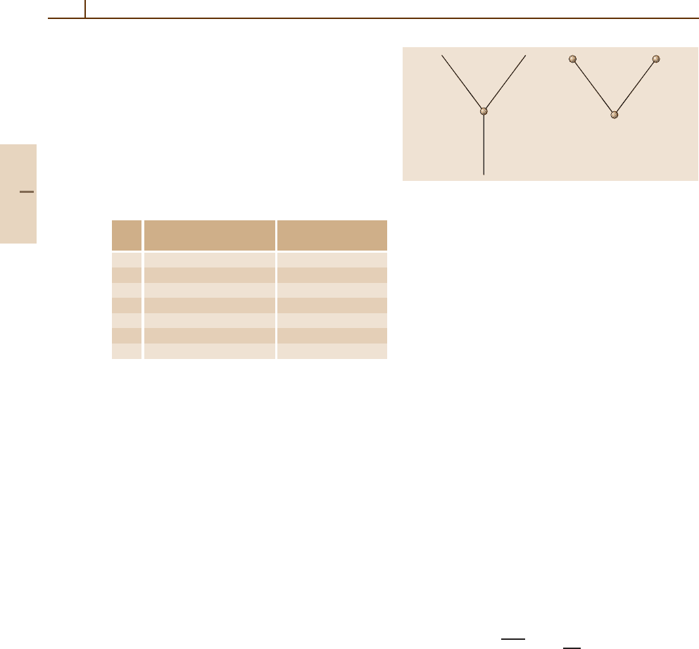
The geometrical object for n = 3 is a planar graph

isomorphic to the tetrahedron in 3-space. The clas-

siﬁcation of all nonisomorphic cubic graphs on

2(n−1) points is an unsolved problem in mathemat-

ics, as is the classiﬁcation of classes for 3(n −1)– j

coefﬁcients.

Fig. 2.4 The fundamental triangle [(ab)c] can be realized

by lines or points

4. There are (at least) two methods of realizing the basic

triangles of angular momentum theory in terms of

graphs. The fundamental structural element [(ab)c]

is represented either in terms of its points or in terms

of its lines (Fig. 2.4):

The right representation leads to the interpretation of

recoupling coefﬁcients as functions deﬁned on pairs

of labeled binary trees [2.1]; the left to the diagrams

of the Jucys school [2.7, 8]. Either method leads to

the relationship of recoupling coefﬁcients to cubic

graphs.

5. The approach of classifying 3n − j coefﬁcients

through the use of unit tensor operator couplings,

Racah operators, 9– j invariant operators, and gen-

eral invariant operators is undeveloped.

2.13 Supplement on Combinatorial Foundations

The quantum theory of angular momentum can be

worked out using the abstract postulates of the prop-

erties of angular momenta operators and the abstract

Hilbert space in which they act. The underlying mathe-

matical apparatus is the Lie algebra of the group SU(2)

and multiple copies thereof. An alternative approach is

to use special Hilbert spaces that realize all the proper-

ties of the abstract postulates and perform calculations

within that framework. The framework must be sufﬁ-

ciently rich in structure so as to apply to a manifold

of physical situations. This approach has been used

often in our treatment; it is an approach that is particu-

larly useful for revealing the combinatorial foundations

of quantum angular momentum theory. We illustrate

this concretely in this supplementary section. The ba-

sic objects are the polynomials deﬁned by (2.24), which

we now call SU(2) solid harmonics, where we change

the notation slightly by interchanging the role of m

and m



2.13.1 SU(2) Solid Harmonics

The SU(2) solid harmonics are deﬁned to be the homo-

geneous polynomials of degree 2 j in four commuting

indeterminates given by



(Z) =

α!β!



(α:A:β)

(2.112)

in which the indeterminates Z and the nonnegative

exponents A are encoded in the matrix arrays

Z =





, A =







i, j=1

, A!=



i, j=1

)!,

α!=α

!α

! ,β!=β

!β

! .

Part A 2.13

Angular Momentum Theory 2.13 Supplement on Combinatorial Foundations 61

The symbol (α : A :β) in (2.112) denotes that the ma-

trix array A of nonnegative integer entries has row and

column sums of its a

entries given in terms of the

quantum numbers j, m, m



= α

= j +m, a

= α

= j −m ,

= β

= j +m



, a

= β

= j −m



These SU(2) solid harmonics are among the most im-

portant functions in angular momentum theory. Not only

do they unify the irreducible representations of SU(2)

in any parametrization by the appropriate deﬁnition of

the indeterminates in terms of generalized coordinates,

they also include the popular boson calculus realiza-

tion of state vectors for quantum mechanical systems,

as well as the state vectors for the symmetric rigid

rotator.

The realization of the inner product is essential.

Physical theory demands an inner product that is given in

terms of integrations of wave functions over the variables

of the theory, as required by the probabilistic inter-

pretation of wave functions. It is the requirement that

realizations of angular momentum operators be Hermi-

tian with respect to the inner product for the spaces being

used that assures the orthogonality of functions, so that

one is able to take results from one realization of the in-

ner product to another with compatibility of relations.

Often, in combinatorial arguments, the inner product

plays no direct role.

The nomenclature SU(2) solid harmonics for the

polynomials deﬁned by (2.112) is by analogy with the

term SO(3, R) solid harmonics for the polynomials

described in Sect. 2.1.

The polynomials Y

(x), x = (x

, x

) ∈ R

are

homogeneous of degree l. The angular momentum op-

erator L

is given by

=−r

∇

+(x·∇)

+(x·∇),

which is a sum of two commuting operators −r

∇

and

(x·∇)

+x·∇, each of which is invariant under orthog-

onal transformations. The SO(3, R) solid harmonics

are homogeneous polynomials of degree l that solve

∇

(x) = 0, so that L

(x) =l(l+1)Y

(x). The

component angular momentum operators L

then have

the standard action on these polynomials, and under real,

proper, orthogonal transformations give the irreducible

representations of the group SO(3, R).

The polynomials D



(Z), z =(z

, z

) ∈

are homogeneous of degree 2 j. The angular mo-

mentum operator J

, with J = (J

, J

),isgiven

=−(det Z)



det

∂

∂Z



+ J

+1),

z·∂ ,

∂ =



∂

∂z

∂

∂z

∂

∂z

∂

∂z



(2.113)

which is a sum of two commuting operators

−(det Z)



det

∂

∂Z



and J

+1), each of which is in-

variant under SU(2) transformations. The SU(2) solid

harmonics are homogeneous polynomials of degree 2 j

such that

det

∂

∂Z



(Z) = 0 ,



(Z) = j( j +1)D



(Z).

The components of the angular momentum op-

erators J = (J

, J

) = (M

, M

) and K =

, K

) then have the standard action on these

polynomials as given in Sect. 2.4.4, and under either

left or right SU(2) transformations these polyno-

mials give the irreducible representations of the

group SU(2).

2.13.2 Combinatorial Deﬁnition

of Wigner–Clebsch–Gordan

Coefﬁcients

The SU(2) solid harmonics have a basic role in

the interpretation of WCG-coefﬁcients in combina-

torial terms. We recall from Sect. 2.7.2 that the

basic abstract Hilbert space coupling rule for com-

pounding two kinematically independent angular mo-

menta with components J

= (J

(1), J

(1)) and

= (J

(2), J

(2)) to a total angular momentum

J =( J

, J

) = J

+ J

|( j

) jm



⊗|j

 . (2.114)

This relation in abstract Hilbert space is realized explic-

itly by spinorial polynomials as follows:

( j

) jm

(Z) =



× ψ

, z

)ψ

, z

(2.115)

Part A 2.13

62 Part A Mathematical Methods

( j

) jm

(Z) =

2 j +1

( j

+ j

− j)!( j

+ j

+ j +1)!

× (det Z)

−j

m, j

−j

(Z),

(2.116)

(x, y) =

j+m

j−m

√

( j +m)!( j −m)!

(2.117)

Explicit knowledge of the WCG-coefﬁcients is not

needed to prove these relationships. The angular mo-

mentum operators

(1) = z

∂

∂z

, J

−

(1) = z

∂

∂z

(1) =



∂

∂z

−z

∂

∂z



;

(2) = z

∂

∂z

, J

−

(2) = z

∂

∂z

(2) =



∂

∂z

−z

∂

∂z



are Hermitian in the polynomial inner product deﬁned

in Sect. 2.4.3, and have the standard action on the

polynomials ψ

, z

) and ψ

, z

), re-

spectively, which are normalized in the inner product

(, ). The components of total angular momentum op-

erator J = M = J

+ J

have the standard action on the

polynomials ψ

( j

) jm

(Z), since they have the standard

action on the factor D

−j

(Z), as given in Sect. 2.4.4,

and [J, det X]=

J, det

∂

∂Z

= 0. Thus, we have

( j

) jm

(Z) = j( j +1)ψ

( j

) jm

(Z),

( j

) jm

(Z) =

( j ∓m)( j ±m +1)

× ψ

( j

) jm±1

(Z).

We also note that the two commuting parts of J

are

diagonal on these functions:

+1)ψ

( j

) jm

(Z)

= ( j

+ j

)( j

+ j

+1)ψ

( j

) jm

(Z),

(det Z)



det

∂

∂X



( j

) jm

(Z)

= ( j

+ j

− j)( j

+ j

+1)ψ

( j

) jm

(Z).

It is necessary only to verify these properties for the

highest weight function D

(Z) = z

2 j

√

(2 j)!, for

which they are seen to hold.

The angular momentum operators K = (K

, K

)

deﬁned in Sect. 2.4.4 with components that commute

with those of J = (M

, M

) and having K

= J

also have a well-deﬁned action on the functions

( j

) jm

(Z). The action of K

, K

−

, and K

on the

quantum numbers ( j

, j

) is to effect the shifts to



, j

−





−

, j



, and ( j

, j

), respec-

tively. These actions of Hermitian angular momentum

operators satisfying the standard commutation relations

K × K = iK are quite unusual in that they depend only

on the angular momentum quantum numbers j

, j

themselves, which satisfy the triangle rule, and give fur-

ther interesting properties of the modiﬁed SU(2) solid

harmonics ψ

( j

) jm

(Z). We note these properties in

full:

( j

) jm

(Z) = j( j +1)ψ

( j

) jm

(Z),

( j

) jm

(Z) = ( j

− j

)ψ

( j

) jm

(Z),

( j

) jm

(Z) =

( j − j

+ j

)( j + j

− j

+1)ψ



−



(Z),

−

( j

) jm

(Z) =

( j + j

− j

)( j − j

+ j

+1)ψ



−



(Z).

These relations play no direct role in our continuing

considerations of (2.116) and the determination of the

WCG-coefﬁcients, and we do not interpret them fur-

ther.

The explicit WCG-coefﬁcients are obtained by ex-

panding the 2 × 2 determinant in (2.116), multiplying

this expansion into the D-polynomial, and changing the

order of the summation. These operations are most suc-

cinctly expressed in terms of the umbral calculus of

Roman and Rota [2.6], using his evaluation operation.

The evaluation at y of a divided power x

/k! of a sin-

gle indeterminate x to a nonnegative integral power k is

deﬁned by

eval

k !

(y)

k !

y(y−1) ···(y−k+1)

k !





where (y)

is the falling factorial. This deﬁnition is

extended to products by

eval

,... ,y

)



i=1



i=1

eval



i=1





It is also extended by linearity to sums of such divided

powers, multiplied by arbitrary numbers.

Part A 2.13

Angular Momentum Theory 2.13 Supplement on Combinatorial Foundations 63

The application of these rules to our problem involv-

ing four indeterminates gives

(det X)



(α:A:α



)



(β:B:β



)

eval



(det X)



(2.118)

β =



+n,α



,β



= (α



+n,α



+n),

eval

(det X)



(−1)







(2.119)

In this result, we do not identify the labels with angu-

lar momentum quantum numbers. Relation (2.119)is

a purely combinatorial, algebraic identity for arbitrary

indeterminates and arbitrary row and column sum con-

straints on the array A as speciﬁed by α =(α

,α

) and







,α





. There are no square roots involved.

We now apply relations (2.118–2.119)tothe

case at hand: n = j

+ j

− j,α= ( j +m, j −m),



= ( j + j

− j

, j − j

+ j

), β = ( j

+ j

+m, j

−m), β



=(2 j

, 2 j

). This gives the following result

for the WCG-coefﬁcients:

( j

+ j

− j)!( j

− j

+ j)!(−j

+ j

+ j)!

( j

+ j

+ j +1)!

(2 j +1)( j +m)!( j −m)!

( j

)!( j

−m

)!( j

−m

×eval

(det X)

−j

( j

+ j

− j)!

(2.120)

eval

(det X)

−j

( j

+ j

− j)!



−j

(−1)









−m



−m



(2.121)

In summary, we have the following:

Up to multiplicative square-root factors, the WCG-

coefﬁcient is the evaluation at the point

B =



−m



of the divided power

(det X)

−j

( j

+ j

− j)!

of a determinant, which is an integer.

The abstract umbral calculus of Rota thus ﬁnds its

way, at a basic level, into angular momentum theory.

Relation (2.120) is but a rewriting in terms of evalua-

tions of the well-known Van der Waerden form of the

WCG-coefﬁcients.

2.13.3 Magic Square Realization

of the Addition

of Two Angular Momenta

The origin of (2.114), giving the states of total angu-

lar momentum by compounding two angular momenta,

is usually attributed to properties of the direct sum of

two copies of the Lie algebra of the unitary unimodular

group SU(2), and to the use of differential operators to

realize the Lie algebras and state vectors, as done above.

It is an interesting combinatorial result that this structure

for adding angular momentum is fully encoded within

the properties of magic squares of order 3, and no opera-

tors whatsoever are needed, only the condition of being

a magic square. We have already noted in Sect. 2.7.4

that Regge observed that the restrictions on the do-

mains of the quantum numbers j

, m

, j

, m

, j, m are

encoded in terms of a magic square A with line-sum

J = j

+ j

+ j :

A =







j −m

−m

j +m

− j

+ jj

− j

+ jj

+ j

− j







(2.122)

The angular momentum quantum numbers are given

in terms of the elements of A = (a

)

1≤i, j≤3

by the

invertible relations

), j

j =

−a

), m

−a

m =

−a

It follows from these deﬁnitions and the fact that A is

a magic square of line-sum J, that the sum rule m

= m and the triangle condition are fulﬁlled.

Part A 2.13

64 Part A Mathematical Methods

We use the symbol j

, j

, j to denote any

triple j

, j

, j of angular momentum quantum num-

bers that satisfy the triangle conditions, where we

note that, if a given triple satisﬁes the triangle

conditions, then all permutations of the triple also

satisfy the triangle conditions. The number of magic

squares for ﬁxed line-sum J is obtained as follows:

Deﬁne ∆

={all triangles j

, j

, j|j

+ j

+ j = J}

and M( j

, j

, j) ={(m

, m

)|−j

≤ m

≤ j

;−j

≤

≤ j

;−j ≤ m

≤ j}. Then we have the fol-

lowing identity, which gives the number of angular

momentum magic squares with line-sum J :



j

, j

, j∈∆

M( j

, j

, j)



J +5



−



J +2



(2.123)

It is nontrivial to effect the summation on the left-hand

side of this relation to obtain the right-hand side, but this

expression is known from the theory of magic squares

Stanley [2.9, 10].

Not only can the addition of two angular momenta in

quantum theory, with its triangle rule for three angular

momentum quantum numbers and its sum rule on the

corresponding projection quantum numbers, be codiﬁed

in magic squares of order 3 and arbitrary line-sum, but

also the content of the abstract state vector of (2.114)

itself can be so expressed:

);

−a

)











C( A)

−a

)

⊗

−a

)

where the summation is over all subsets





of the magic square of order 3 such that row 3 and column

3 are held ﬁxed. The coefﬁcients C(A) themselves are

the WCG-coefﬁcients, which may be regarded as a func-

tion whose domain of deﬁnition is the set of all magic

squares of order 3. The triangle rule j

, j

, j and the

sum rule on (m

, m

, m) are implied by the structure of

magic squares of order 3. These rich combinatorial foot-

ings of angular momentum theory are completed by the

observation that the Clebsch–Gordan coefﬁcients them-

selves are obtained by the Schwinger–Regge generating

function given in Sect. 2.7.3 (see [2.2] for the relation to

hypergeometric functions).

2.13.4 MacMahon’s and Schwinger’s

Master Theorems

Generating functions codify the content of many math-

ematical entities in a unifying, comprehensive way.

These functions are very popular in combinatorics, and

Schwinger used them extensively in his treatment of an-

gular momentum theory. In this subsection, we present

a natural generalization of the SU(2) solid harmonics to

a class of polynomials that are homogeneous in n

in-

determinates. While these polynomials are of interest in

their own right, it is their fundamental role in the ad-

dition of n kinematically independent angular momenta

that motivates their introduction here. They bring an

unexpected unity and coherence to angular momentum

coupling and recoupling theory [2.11].

We list in compendium format some of the principal

results:

Special U(n) solid harmonics:

α,β

(Z) =

α!β!



A∈M(α,β)

(2.124)

A = (a

)

1≤i, j≤n

: matrix of order n in nonnegative inte-

gers;

A!=



i, j=1

! , Z



i, j=1

;

where we employ the notations:

α = (α

,α

,... ,α

): sequence (composition) of non-

negative integers having the sum k, denoted α  k;

= x

···x

,α!=α

!α

!···α

β =(β

,β

,... ,β

): second composition β  k ;

M(α, β), set of all matrices A such that the entries in

row i sums to α

and those in column j to β

The signiﬁcance of the row-sum vector α is that

is the degree of the polynomial in the variables

, z

,... ,z

) in row i of Z, with a similar inter-

pretation for β in terms of columns.

Matrix of the D

α,β

(Z) polynomials:

The number of compositions of the integer k into n non-

negative parts is given by



n+k−1



. The compositions in

this set may be linearly ordered by the lexicograph-

ical rule α>β, if the ﬁrst nonzero part of α −β is

Part A 2.13

Angular Momentum Theory 2.13 Supplement on Combinatorial Foundations 65

positive. The polynomial D

α,β

(Z) is then the entry

in row α and column β in the matrix D

(Z) of di-

mension dim D

(Z) =



n+k−1



, where, following the

convention for SU(2), the rows are labelled from top

to bottom by the greatest to the least sequence, and the

columns are labelled in the same manner as read from

left to right. There is a combinatorial proof by Chen and

Louck[2.12] that these polynomials satisfy the following

multiplication rule for arbitrary matrices X and Y:

(XY ) = D

(X)D

(Y). (2.125)

Orthogonality in the inner product (, )deﬁned

in Sect. 2.4.3:

α,β

, D



,β



= δ

α,α



β,β



k ! .

Val ue o n Z = diag(z

, z

,... ,z

) :

α,β

diag(z

, z

,... ,z

)

= δ

α,β

, (2.126)

) = I



n+k−1



Transposition property:

) =

(Z)

Special irreducible unitary representations of U(n) :

(U)D

(V) = D

(UV), all U, V ∈U(n).

Schwinger’s Master Theorem: For any two matrices X

and Y of order n, the following identities hold:

(∂

:X:∂

)

(x:Y:y)

x=y=0

∞



k=0



α,βk

α,β

(X)D

β,α

(Y)

det(I − XY )

(2.127)

(x : Z : y) = xZy



i, j=1

MacMahon’s Master Theorem: Let X be the diagonal

matrix X = diag(x

, x

,... ,x

) and Y amatrixofor-

der n. Then the coefﬁcient of x

in the expansion of

det(I−XY)

equals the coefﬁcient of x

in the product

, y

j=1

, that is,

det(I − XY)

∞



k=0



αk

α,α

(Y) x

. (2.128)

Basic Master Theorem: Let Z be a matrix of order n.

Then

det(I −tZ)

∞



k=0



αk

α,α

(Z). (2.129)

Schwinger’s relation (2.127) follows from the ba-

sic relation (2.129) by setting Z = XY and using

the multiplication property (2.125); MacMahon’s rela-

tion then follows from Schwinger’s result by setting

X = diag(x

, x

,... ,x

) and using property (2.126).

Of course, MacMahon’s Master Theorem preceded

Schwinger’s result by many years (see MacMa-

hon [2.13]).The uniﬁcation into the single form by using

properties of the D

α,β

(Z) polynomials was pointed out

in [2.14]. More surprisingly, relation (2.129) was al-

ready discovered for the general linear group in 1897 by

Molien [2.15]; its properties are developed extensively

in Michel and Zhilinski [2.16] in the context of group

theory.

For many purposes, it is better in combinatorics to

avoid all square roots by using the polynomials

α,β

(Z) =



A∈M(α,β)

in place of the D

α,β

(Z) deﬁned in (2.124).

2.13.5 The Pfafﬁan and Double Pfafﬁan

Schwinger observed that the calculation of 3n − j coefﬁ-

cients involves taking the square root

√

(I − AB), where

A and B are skew symmetric (antisymmetric) matrices

of order n, but the procedure is rather obscure. The ap-

propriate concepts for taking the square root is that of

a Pfafﬁan and a double Pfafﬁan, denoted, respectively,

by Pf(A) and Pf(A, B). The deﬁnitions require the con-

cept of a matching of the set of integers {1, 2,... ,n}.

A matching of {1, 2,... ,n} is an unordered set of

disjoint subsets {i, j} containing two elements. For ex-

ample, the matchings of 1, 2, 3are{1, 2}, {1, 3}, and

{2, 3}. We then have the following constructs:

Pfafﬁan and double Pfafﬁan of skew symmetric matrices

A = (a

) and B =(b

) of order n :

Pf(A) =



},{i

},... ,{i

n−1

}

ε(i

···i

)

× a

···a

n−1

, (2.130)

Part A 2.13

66 Part A Mathematical Methods

Pf(A, B) = 1 +



k≥1



, i

}, {i

, i

},... ,{i

2k−1

, i

}

, j

}, {j

, j

},... ,{j

2k−1

, j

}

ε(i

·i

)ε( j

···j

)

× a

···a

2k−1

× b

, j

···b

2k−1

, j

(2.131)

where {i

, i

}, {i

, i

},... ,{i

n−1

, i

} is a matching of

{1, 2,... ,n},and ε(i

···i

) is the sign of the permu-

tation (number of inversions). Similarly, in the double

Pfafﬁan, the 2-subsets are matchings of a subset of

{1, 2,... ,n} of even length.

Relations of skew symmetric matrices A, B to Pfafﬁans:

√

det A =Pf(A) ;

det(I − AB) = Pf(A, B).

(2.132)

2.13.6 Generating Functions

for Coupled Wave Functions

and Recoupling Coefﬁcients

This section is a reformulation, nontrivial extension, and

interpretation of results found in Schwinger [2.3]. We

ﬁrstreﬁnethenotationusedinSect.2.12.3.

Set of triangles in the coupling scheme:

Each coupling scheme, as determined by the bracketing

B, has associated with it a unique ordered set of n −1

triangles

( j, k, j) ={a

, b

, k

|i = 1, 2,... ,n −1} ,

j = ( j

, j

,... , j

k = (k

, k

,... ,k

n−2

n−1

= j .

The third part k

of a

, b

, k

 can always be chosen,

without loss of generality, as an intermediate angu-

lar momentum (k

n−1

= j), and the triangles in the set

can be ordered by a

, b

, k

 < a

i+1

, b

i+1

, k

i+1

. The

remaining pair of angular momentum labels in the tri-

angle a

, b

, k

 then fall, in general, into four classes:

a

, b

, k

 in which a

can be either a j

or a k

,andb

can be either a j



or k



. The distribution of the j



s and



s among the a

and b

is uniquely determined by the

bracketing B that deﬁnes the coupling scheme.

Clebsch–Gordan coefﬁcients for a given coupling

scheme:



jkj

mqm





a

∈T

( j,k, j)

, (2.133)

in which the projection quantum numbers α

and

are m



s and q



s that match the a

and b

In the given coupling scheme determined by the

bracketing B, only ( j

, m

), i =1, 2 ... ,n;(k

, q

), i =

1, 2,...,n −2, and ( j, m) appear in the Clebsch–

Gordan coefﬁcients. In fact, if one explicitly implements

the sum rule on the projection quantum numbers, it is

always possible to express the q

as sums over the m

and m.

Coupled angular momentum function for n angular

momenta:

( jk) jm

(x, y) =





jkj

mqm





i=1

, y

(2.134)







··· j

··· m









··· k

n−2

··· q

n−2



(2.135)

Z = (z

...z

n+1

) =



... x

n+1

... y

n+1



(2.136)

Only the ﬁrst n columns of Z enter into (2.136), but the

last column occurs below.

The skew symmetric matrix of a coupling scheme:

The set of triangles T

( j, k, j) ={a

, b

, k

|i =

1, 2,... ,n−1}, which is uniquely deﬁned by the brack-

eting B, can be mapped to a unique skew symmetric

matrix of order n +1. This mapping is one of the most

important results for obtaining generating functions for

the coupled wave functions (2.134) and the recoupling

coefﬁcients given below. The skew symmetric matrix

depends on the bracketing B and the detailed man-

ner in which the j



s and k



s are distributed among the

triangles in T

( j, k, j). The rule for constructing the

skew symmetric matrix is quite intricate. First, we deﬁne

a3×(n −1) matrix T of indeterminates by

T =







··· t

1,n−1

··· t

2,n−1

··· t

3,n−1







(2.137)

Second, we associate with each a

, b

, k

∈

( j, k, j), a triple of indeterminates (u

) as

Part A 2.13

Angular Momentum Theory 2.13 Supplement on Combinatorial Foundations 67

given by

a

, b

, k

→(u

), with w

a

, b

, k

→(u

), with w

a

n−1

, b

n−1

, k

n−1

 → (u

n−1

with w

n−1

= t

2,n−1

n−2

1,n−1

n−1

. (2.138)

The indeterminates u

and v

are identiﬁed as a col-

umn z

= (x

, y

) of the 2 × (n +1) matrix Z deﬁned

by (2.136), or as one of the w



s occurring higher in the

display (2.138). The distribution rule is in one-to-one

correspondence with the distribution of j



s and k



s in

the corresponding triangle. Thus, we have

= z

, if a

= j

; v

= z

, if b

= j

;

= z

, if a

= j

; v

= w

, if b

= k

;

= w

, if a

= k

; v

= z

, if b

= j

;

= w

, if a

= k

; v

= w

, if b

= k

The explicit identiﬁcation of all j



s and k



s is uniquely

determined by the bracketing B. Once this identiﬁcation

has been made, the elements a

, i < j of the skew sym-

metric matrix A of order n +1 are uniquely determined

in terms of the elements of T by equating coefﬁcients of

det(z

, z

) = x

−x

on the two sides of the form



1≤i< j≤n+1

det(z

, z

)

n−1



i=1

det(u

) +det(w

n−1

, z

n+1

), (2.139)

where (t

, t

) is the i-th column of the 3 × (n −1)

matrix T of indeterminates. This relation can be inferred

from results given by Schwinger. Since the elements of

A are determined as monomials in the elements of T, we

sometimes denote A by A(T).

It is useful to illustrate the rule for determining A for

n = 2, 3, 4:

n = 2: Triangle: j

, j

, k

:

= t

det(z

, z

) +a

det(z

, z

) +a

det(z

, z

)

= t

det(u

) +det(w

, z

)

= t

det(z

, z

) +t

det(z

, z

)

det(z

, z

) ;

= t

, a

= t

, a

= t

n = 3: Ordered triangles: j

, j

, k

, k

, j

, k

:

= t

, u

= z

;

= t

, u

= w

= z



1≤i< j≤4

det(z

, z

)

= t

det(u

) +t

det(u

) +det(w

, z

) ;

= t

, a

= t

, a

= t

, a

= t

n = 4: Ordered triangles: j

, j

, k

, j

, j

, k

,

k

, k

:

= t

, u

= z

= t

, u

= z

= t

, u

= w

;

= t



1≤i< j≤5

det(z

, z

) = t

det(u

) +t

×det(u

) +t

det(u

) +det(w

, z

) ;

= t

, a

=−t

, a

= t

=−t

, a

=−t

= t

Triangle monomials:

Let a, b, c be a triangle of quantum numbers

(a, b, c),let(x, y, z) be three indeterminates, and let B

denote a binary coupling scheme with the set of triangles

( j, k, j) :

Elementary triangle monomial:

a,b,c

(x, y, z) ={abc}

−1

b+c−a

a+c−b

a+b−c

(2.140)

{abc}



(2c+1)(b+c−a)(a+c−b)!(a+b−c)!

(a+b+c+1)!



Triangle monomial associated with a given coupling

scheme B :

j,k, j

(T ) =



a

∈T

( j,k, j)

a



, t

(2.141)

Part A 2.13