Drake G.W.F. (editor) Handbook of Atomic, Molecular, and Optical Physics
Подождите немного. Документ загружается.


48 Part A Mathematical Methods
form:
abc
ρστ
=
αβγ
C
abc
αβγ
*
a+ρ
2a 0
a+α
+
1
⊗
*
b+σ
2b 0
b+β
+
2
*
c+τ
2c 0
c+γ
+
†
. (2.90)
This form is taken as the definition of the 9– j invariant
operator. Its eigenvalues in the coupled basis define the
9– j coefficient:
abc
ρστ
|( j
1
j
2
) jm
=( j
1
+ρ, j
2
+σ) j +τ|
&
&
&
&
&
abc
ρστ
&
&
&
&
&
|( j
1
j
2
) j
× |( j
1
j
2
) jm
=[(2 j +1)(2c+1)(2 j
1
+2ρ +1)(2 j
2
+2σ +1)]
1
2
×
j
1
j
2
j
abc
j
1
+ρ j
2
+σ j +τ
|( j
1
j
2
) jm . (2.91)
The 9– j invariant operators play exactly the same role
in the tensor product space of two irreducible angular
momentum spaces as do the Racah invariants in one such
irreducible angular momentum space.
The full content of the coupling law (2.86b)for
physical irreducible tensor operators is regained in the
coupling law for reduced matrix elements:
4
α
1
α
2
j
1
j
2
j
5
5
[T
a
(1) × T
b
(2)]
c
5
5
(α
1
α
2
j
1
j
2
) j
-
=
j
1
j
2
j
abc
j
1
j
2
j
4
α
1
j
1
5
5
T
a
(1)
5
5
(α
1
) j
1
-
×
4
α
2
j
2
5
5
T
b
(2)
5
5
(α
2
) j
2
-
;
(2.92a)
j
1
j
2
j
abc
j
1
j
2
j
=
!
2 j
1
+1
2 j
2
+1
(2 j +1)(2c+1)
"
1
2
×
j
1
j
2
j
abc
j
1
j
2
j
.
(2.92b)
2.10.3 Basic Relations Between 9– j
Coefficients and 6– j Coefficients
Orthogonality of 9– j coefficients:
hi
(2c+1)(2 f +1)(2h +1)(2i+1)
×
abc
def
hi j
abc
def
hi j
= δ
cc
δ
ff
,
where this relation is to be applied only to triples (abc),
(def ), (cfj), (abc
), (def
), (c
f
j) for which the triangle
conditions hold.
9– j coefficients in terms of 3– j coefficients:
δ
j
33
j
33
(2 j
33
+1)
−1
j
11
j
12
j
13
j
21
j
22
j
23
j
31
j
32
j
33
=
all m
ij
except m
33
j
11
j
12
j
13
m
11
m
12
m
13
j
21
j
22
j
23
m
21
m
22
m
23
×
j
31
j
32
j
33
m
31
m
32
m
33
j
11
j
21
j
31
m
11
m
21
m
31
×
j
12
j
22
j
32
m
12
m
22
m
32
j
13
j
23
j
33
m
13
m
23
m
33
.
(2.93)
9– j coefficients in terms of 6– j coefficients:
j
11
j
12
j
13
j
21
j
22
j
23
j
31
j
32
j
33
=
k
(−1)
2k
(2k+1)
×
j
11
j
21
j
31
j
32
j
33
k
j
12
j
22
j
32
j
21
kj
23
×
j
13
j
23
j
33
kj
11
j
12
.
(2.94)
Basic defining relation for 9– j coefficient from (2.88):
(−1)
φ
j
12
j
22
j
32
j
11
j
21
j
31
j
13
j
23
j
33
j
31
j
32
j
33
m
31
m
32
m
33
=
all m
(1i)
m
(2i)
j
11
j
21
j
31
m
11
m
21
m
31
Part A 2.10

Angular Momentum Theory 2.10 The 9–j Coefficients 49
×
j
12
j
22
j
32
m
12
m
22
m
32
j
13
j
23
j
33
m
13
m
23
m
33
×
j
11
j
12
j
13
m
11
m
12
m
13
j
21
j
22
j
23
m
21
m
22
m
23
,
φ =
kl
j
kl
. (2.95)
Additional relations:
kl
(−1)
2b+l+h− f
(2k+1)(2l+1)
×
abc
ed f
kli
aek
dbl
ghi
=
abc
def
gh i
,
c
(2c+1)
abc
def
gh i
abc
fij
= (−1)
2 j
def
bjh
ghi
jad
,
klm
(2k+1)(2l+1)(2m +1)
×
abc
de f
klm
klm
a
b
c
d
e
f
×
adk
a
d
k
bel
b
e
l
cfm
c
f
m
=
abc
d
e
f
k
l
m
k
l
m
a
b
c
de f
.
2.10.4 Symmetry Relations
for 9– j Coefficients and Reduction
6– j Coefficients
The 9– j coefficient
j
11
j
12
j
13
j
21
j
22
j
23
j
31
j
32
j
33
is invariant under even permutation of its rows, even per-
mutation of its columns, and under the interchange of
rows and columns (matrix transposition). It is multiplied
by the factor (−1)
φ
(2.95) under odd permutations of its
rows or columns. These 72 symmetries are all conse-
quences of the 72 symmetries of the 3– j coefficient in
relation (2.93).
Reductionto6–j coefficients:
abe
cde
ff0
=
0 ee
fdb
fca
=
e 0 e
cfa
dfb
=
ff0
dce
bae
=
fbd
0 ee
fac
=
afc
e 0 e
bfd
=
bae
ff0
dce
=
edc
eba
0 ff
=
ced
aeb
f 0 f
=
(−1)
b+c+e+f
[(2e+1)(2 f +1)]
1
2
abe
dcf
.
2.10.5 Explicit Algebraic Form
of 9– j Coefficients
abc
def
hi j
= (1)
c+f −j
(dah)(bei)( jhi)
(def )(bac)( jcf )
×
xyz
(−1)
x+y+z
x!y!z!
×
(2 f −x)!(2a−z)!
(2i +1 +y)!(a+d +h +1 −z)!
×
(d+e− f +x)!(c+ j− f +x)!
(e+ f −d−x)!(c+ f − j−x)!
×
(e+i −b+ y)!(h +i − j+y)!
(b+e−i −y)!(h + j−i −y)!
×
(b+c−a+z)!
(a+d−h −z)!(a+c−b−z)!
×
(a+d+ j −i −y−z)!
(d+i −b− f +x +y)!(b+ j −a− f +x +z)!
,
(abc)
=
(a−b+c)!(a+b−c)!(a+b+c+1)!
(b+c−a)!
1
2
.
Part A 2.10

50 Part A Mathematical Methods
2.10.6 Racah Operators
A Racah operator is denoted
a+ρ
2a 0
a+σ
ρ, σ = a, a−1,... ,−a,
2a = 0, 1, 2,... ,
and is a special case of the operator defined by (2.87):
a+ρ
2a 0
a+σ
|( j
1
j
2
) jm
=
(2a+1)(2 j
2
+1)
(2 j
2
+2σ +1)
1
2
T
(aa)0
(ρσ)0
|( j
1
j
2
) jm . (2.96)
Thus, a Racah operator is an invariant operator with
respect to the total angular momentum J. Alternative
definitions are:
a+ρ
2a 0
a+σ
= (−1)
a+σ
a
*
a+ρ
2a 0
a+α
+
⊗
*
a−σ
2a 0
a+α
+
†
,
a+ρ
2a 0
a+σ
&
&
( j
1
j
2
) jm
-
=[(2 j
1
+2ρ +1)(2 j
2
+1)]
1
2
× W( j, j
1
, j
2
+σ, a; j
2
, j
1
+ρ)
× |( j
1
+ρ, j
2
+σ) jm
with conjugate
a+ρ
2a 0
a+σ
†
&
&
( j
1
j
2
) jm
-
=[(2 j
1
+1)(2 j
2
−2σ +1)]
1
2
× W( j, j
1
−ρ, j
2
, a; j
2
−σ, j
1
)
× |( j
1
−ρ, j
2
−σ) jm .
Racah operators satisfy orthogonality relations similar
in form to Wigner operators. The open product rule
is:
b+σ
2b 0
b+β
a+ρ
2a 0
a+α
=
c
W
abc
ρ,σ,ρ+σ
W
abc
α,β,α+β
c+ρ +σ
2c 0
c+α +β
.
(2.97)
In this result W
abc
ρστ
and W
abc
α,β,α+β
denote Racah invari-
ants with respect to the angular momenta J(1) and J(2),
respectively, so that
W
abc
ρστ
|( j
1
j
2
) jm=W
abc
ρστ
( j
1
)|( j
1
j
2
) jm ,
W
abc
αβγ
|( j
1
j
2
) jm=W
abc
αβγ
( j
2
)|( j
1
j
2
) jm .
The matrix elements of relation (2.97) lead to the
Biedenharn–Elliott identity. There are five versions of
this relationship in complete analogy to relations (2.63–
2.65)and(2.69–2.70) for Wigner operators.
Racah operators are a basis for all invariant opera-
tors acting in the tensor product space spanned by the
coupled basis vectors (2.85) and are the natural way of
formulating interactions in that space. Their algebra is
a fascinating study, initiated already in a different guise
in the work of Schwinger [2.3]. Little use has been made
of this concept in physical applications.
Additional relations between Racah coefficients or
6– j coefficients may be derived from the various ver-
sions of the rule (2.97) or directly from relation (2.79b)
by using the orthogonality relations (2.75). Two of these
are:
e
(−1)
a+b+e
(2e+1)
×
abe
dcg
a
ac
bb
e
a
eb
dd
c
= (−1)
φ
1
c
bb
dd
g
a
ac
gd
c
,
φ
1
= g+a
+b
+c
+c+d
+d ;
e,e
(−1)
a−c
+e−e
(2e+1)(2e
+1)(2 f +1)
×
c
be
dd
f
abe
dcg
a
ac
be
e
a
ee
dd
c
= δ
fg
(−1)
φ
2
a
ac
gd
c
,
φ
2
= g+a
−b+c+d
+d .
Part A 2.10
Angular Momentum Theory 2.10 The 9–j Coefficients 51
The W-coefficient form of these relations is obtained
by deleting all phase factors and making the sub-
stitution (2.74), ignoring the phase factor. There are
no phase factors in the corresponding W-coefficient
relations.
2.10.7 Schwinger–Wu Generating Function
and its Combinatorics
Triangles associated with the 9– j coefficient
j
1
j
2
j
3
j
4
j
5
j
6
j
7
j
8
j
9
:
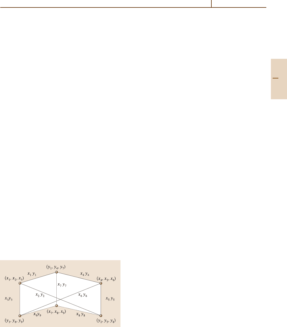
( j
1
j
2
j
3
), (j
4
j
5
j
6
), (j
7
j
8
j
9
), (j
1
j
4
j
7
),
( j
2
j
5
j
8
), (j
3
j
6
j
9
).
Points in R
3
associated with the triangles:
( j
1
j
2
j
3
) → (x
1
, x
2
, x
3
), ( j
4
j
5
j
6
) → (x
4
, x
5
, x
6
),
( j
7
j
8
j
9
) → (x
7
, x
8
, x
9
), ( j
1
j
4
j
7
) → (y
1
, y
4
, y
7
),
( j
2
j
5
j
8
) → (y
2
, y
5
, y
8
), ( j
3
j
6
j
9
) → (y
3
, y
6
, y
9
).
Cubic graph C
6
in R
3
associated with the points:
The points define the vertices of a cubic graph C
6
on six points with lines joining each pair of points
that share a common subscript, and the lines are la-
beled by the products x
i
y
i
,wherei is the common
subscript (Fig. 2.3).
Cubic graph C
6
functions:
Interchange the symbols x and y in the coordinates
of the vertices of the cubic graph C
6
, and define the fol-
lowing polynomials on the vertices and edges of the C
6
with this modified labeling:
Vertex function: multiply together the coordinates of
each pair of adjacent vertices, divide out the coordinates
with a common subscript, and sum over all pairs of
Fig. 2.3 Labeled cubic graph associated with the 9– j coef-
ficient
vertices to obtain
V
4
= y
1
y
2
x
6
x
9
+y
1
y
3
x
5
x
8
+y
2
y
3
x
4
x
7
+y
4
y
5
x
3
x
9
+y
4
y
6
x
2
x
8
+y
5
y
6
x
1
x
7
+y
7
y
8
x
3
x
6
+y
7
y
9
x
2
x
5
+y
8
y
9
x
1
x
4
.
Edge function:
E
6
= det
x
1
y
1
x
2
y
2
x
3
y
3
x
4
y
4
x
5
y
5
x
6
y
6
x
7
y
7
x
8
y
8
x
9
y
9
.
Generating function [2.4–6]:
(1 −V
4
+E
6
)
−2
=
∆
C(∆)Z
∆
,
Z
∆
=
all vertices
(z
a
, z
b
, z
c
)
( j
a
j
b
j
c
)
[see (2.82,)],
∆ =
( j
1
j
2
j
3
)
( j
4
j
5
j
6
)
( j
7
j
8
j
9
)
( j
1
j
4
j
7
)
( j
2
j
5
j
8
)
( j
3
j
6
j
9
)
,
C(∆) =
k
a
(−1)
k
10
+k
11
+k
12
(k+1)
×
k
k
1
,... ,k
9
, k
10
,... ,k
15
,
where summation
8
is over all 3 × 3 square arrays of
nonnegative integers k
j
( j = 1, 2,... ,9) with fixed row
and column sums given by
k
1
k
2
k
3
k
4
k
5
k
6
k
7
k
8
k
9
k−t
4
k−t
5
k−t
6
k−t
1
k−t
2
k−t
3
and for each such array the summation
8
a
is over all
nonnegative integers a such that the following quantities
are nonnegative integers:
k
10
=−a+k
1
−k+ j
2
+ j
3
+ j
4
+ j
7
,
k
11
=−a+k
6
−k+ j
3
+ j
4
+ j
5
+ j
9
,
k
12
=−a+k
8
−k+ j
2
+ j
5
+ j
7
+ j
9
,
k
13
= a+k
5
−k
1
− j
3
+ j
6
− j
7
+ j
8
,
k
14
= a+k
2
−k
6
+ j
1
− j
4
+ j
8
− j
9
,
k
15
= a .
Part A 2.10

52 Part A Mathematical Methods
Note that
15
i=10
k
i
=−2k+
9
i=1
j
i
.
The t
i
are the following triangle sums:
t
1
= j
1
+ j
2
+ j
3
, t
2
= j
4
+ j
5
+ j
6
,
t
3
= j
7
+ j
8
+ j
9
,
t
4
= j
1
+ j
4
+ j
7
, t
5
= j
2
+ j
5
+ j
8
,
t
6
= j
3
+ j
6
+ j
9
.
The 9– j coefficient is given by
j
1
j
2
j
3
j
4
j
5
j
6
j
7
j
8
j
9
= ∆( j
1
j
2
j
3
)∆( j
4
j
5
j
6
)∆( j
7
j
8
j
9
)
× ∆( j
1
j
4
j
7
)∆( j
2
j
5
j
8
)∆( j
3
j
6
j
9
)C(∆) .
The coefficient C(∆) is an integer associated with
each cubic graph C
6
that counts the number of occur-
rences of the monomial term Z
∆
in the expansion of
(1 −V
4
+E
6
)
−2
.
2.11 Tensor Spherical Harmonics
Tensor spherical or tensor solid harmonics are special
cases of the coupling of two irreducible tensor operators
in the tensor product space given in Sect. 2.7.2.Theyare
defined by
Y
(ls) jm
=
ν
C
lsj
m−ν,ν,m
Y
l,m−ν
⊗ξ
ν
and belong to the tensor product space H
l
⊗H
s
,where
the orthonormal bases of the spaces H
l
and H
s
are:
(
Y
lµ
: µ =l, l −1,... ,−l
)
,
{
ξ
ν
: ν =s, s−1,... ,−s
}
.
The orbital angular momentum Lhas the standard action
on the solid harmonics, and a second set of kinemati-
cally independent angular momentum operators S has
the standard action on the basis set of H
s
.
The total angular momentum is:
J = L⊗1
+1 ⊗S,
The set of vectors
{
Y
(ls) jm
: m = j, j −1,... ,−j;(lsj)
obey the triangle conditions
}
has the following following properties:
Orthogonality:
%
Y
(l
s) j
m
, Y
(ls) jm
'
=
νν
C
l
sj
m
−ν
,ν
,m
C
lsj
m−ν,ν,m
(Y
l
,m
−ν
,
Y
l,m−ν
)
× (ξ
ν
,ξ
ν
)
= δ
j
j
δ
l
l
δ
m
m
,
where
,
denotes the inner product in the space
H
l
⊗H
s
,(, ) the inner product in H
l
,and(, )
the
inner product in H
s
.
Operator actions:
J
2
Y
(ls) jm
= j( j +1)Y
(ls) jm
,
J
3
Y
(ls) jm
= mY
(ls) jm
,
(L
2
⊗1
)Y
(ls) jm
=l(l+1)Y
(ls) jm
,
(1 ⊗S
2
)Y
(ls) jm
= s(s+1)Y
(ls) jm
,
J
2
= L
2
⊗1
+1 ⊗S
2
+2
i
L
i
⊗S
i
,
J
±
Y
(ls) jm
=[( j ∓m)( j ±m +1)]
1
2
Y
(ls) j,m±1
.
Transformation property under unitary rotations:
exp(−iψ
ˆ
n· J)Y
(ls) jm
=
m
D
j
m
m
(ψ,
ˆ
n)Y
(ls) jm
.
Special realization:
The eigenvectors ξ
ν
are often replaced by column
matrices:
ξ
ν
= col(0 ···010 ···0),
1 in position s−ν +1,ν= s, s−1,... ,−s .
The operators S =(S
1
, S
2
, S
3
) are correspondingly re-
placed by their standard (2s+1) × (2s +1) matrix
representations S
(s)
i
. The tensor product of operators
becomes a (2s +1) × (2s+1) matrix containing both
operators and numerical matrix elements, e.g.,
J
i
= L
i
I
2s+1
+S
(s)
i
,
in which L
i
is a differential operator multiplying the
unit matrix, that is, L
i
is repeated 2s+1 times along the
diagonal.
Part A 2.11
Angular Momentum Theory 2.11 Tensor Spherical Harmonics 53
2.11.1 Spinor Spherical Harmonics
as Matrix Functions
Choose ξ
+1/2
= col(1, 0), ξ
−1/2
= col(0, 1),andS =
σ/2. The spinor spherical harmonics or Pauli
central field spinors are the following, where
j ∈
{
1/2, 3/2,...
}
:
Y
j−
1
2
,
1
2
jm
=
9
j+m
2 j
Y
j−
1
2
,m−
1
2
9
j−m
2 j
Y
j−
1
2
,m+
1
2
,
Y
j+
1
2
,
1
2
jm
=
−
9
j−m+1
2 j+2
Y
j+
1
2
,m−
1
2
9
j+m+1
2 j+2
Y
j+
1
2
,m+
1
2
.
2.11.2 Vector Spherical Harmonics
as Matrix Functions
Choose ξ
+1
= col(1, 0, 0), ξ
0
= col(0, 1, 0), ξ
−1
=
col(0, 0, 1), and Sthe 3 × 3 angular momentum matrices
given by
S
+
=
0
√
20
00
√
2
00 0
, S
−
=
000
√
200
0
√
20
,
S
3
=
10 0
00 0
00−1
.
The vector spherical harmonics are the following, where
j ∈
{
0, 1, 2,...
}
:
Y
( j−1,1) jm
=
9
( j+m−1)( j+m)
2 j(2 j−1)
Y
j−1,m−1
9
( j−m)( j+m)
j(2 j−1)
Y
j−1,m
9
( j−m−1)( j−m)
2 j(2 j−1)
Y
j−1,m+1
,
Y
( j1) jm
=
−
9
( j+m)( j−m+1)
2 j( j+1)
Y
j,m−1
m
√
j( j+1)
Y
j,m
9
( j−m)( j+m+1)
2 j( j+1)
Y
j,m+1
,
Y
( j+1,1) jm
=
9
( j−m+1)( j−m+2)
2( j+1)(2 j+3)
Y
j+1,m−1
−
9
( j−m+1)( j+m+1)
( j+1)(2 j+3)
Y
j+1,m
9
( j+m+2)( j+m+1)
2( j+1)(2 j+3)
Y
j+1,m+1
.
Eigenvalue properties:
∇
2
Y
(l1) jm
= 0 ,
J
2
Y
(l1) jm
= j( j +1)Y
(l1) jm
,
J
3
Y
(l1) jm
= mY
(l1) jm
,
L
2
Y
(l1) jm
=l(l+1)Y
(l1) jm
,
S
2
Y
(l1) jm
= 2Y
(l1) jm
.
2.11.3 Vector Solid Harmonics
as Vector Functions
Vector spherical and solid harmonics can also be defined
and their properties presented in terms of the ordinary
solid harmonics, using the vectors x, ∇, and L,andthe
operations of divergence and curl:
Defining equations:
Y
(l+1,1)lm
=−[(l+1)(2l+1)]
−
1
2
[(l+1)x
+ix× L]Y
lm
,
Y
(l1)lm
=[l(l+1)]
−1/2
LY
lm
,
r
2
Y
(l−1,1)lm
=−[l(2l+1)]
−
1
2
× (−lx+ix
× L)Y
lm
.
Eigenvalue properties:
J
2
Y
(l1) jm
= j( j +1)Y
(l1) jm
,
L
2
Y
(l1) jm
=l(l+1)Y
(l1) jm
,
S
2
Y
(l1) jm
= 2Y
(l1) jm
,
J
3
Y
(l1) jm
= mY
(l1) jm
,
∇
2
Y
(l1) jm
= 0 ,
2iL× Y
(l1) jm
=[j( j +1) −l(l+1) −2]Y
(l1) jm
.
Orthogonality:
dS
ˆ
x
Y
(l
1) j
m
∗
(x) ·Y
(l1) jm
(x) = δ
l
l
δ
j
j
δ
m
m
r
l
+l
,
where the integration is over the unit sphere in R
3
.
Complex conjugation:
Y
(l1) jm∗
= (−1)
l+1−j
(−1)
m
Y
(l1) j,−m
.
Part A 2.11

54 Part A Mathematical Methods
Vector and gradient formulas:
xY
lm
=−
l+1
2l+1
1
2
Y
(l+1,1)lm
+
l
2l+1
1
2
r
2
Y
(l−1,1)lm
,
[(l+1)∇+i∇× L](FY
lm
)
=−[(l+1)(2l+1)]
1
2
1
r
dF
dr
Y
(l+1,1)lm
,
[−l∇+i∇ × L](FY
lm
)
=−[l(2l+1)]
1
2
r
dF
dr
+(2l+1)F
Y
(l−1,1)lm
,
∇(FY
lm
) =−
l+1
2l+1
1
2
1
r
dF
dr
Y
(l+1,1)lm
+
l
2l+1
1
2
r
dF
dr
+(2l+1)F
Y
(l−1,1)lm
,
i∇× L(FY
lm
) =−l
l+1
2l+1
1
2
1
r
dF
dr
Y
(l+1,1)lm
−(l+1)
l
2l+1
1
2
×
r
dF
dr
+(2l+1)F
Y
(l−1,1)lm
.
Curl equations:
i∇× (FY
(l+1,1)lm
) =−
l
2l+1
1
2
×
r
dF
dr
+(2l+3)F
Y
(l1)lm
,
i∇× (FY
(l1)lm
) =−
l
2l+1
1
2
×
1
r
dF
dr
Y
(l+1,1)lm
−
l+1
2l+1
1
2
×
r
dF
dr
+(2l+1)F
Y
(l−1,1)lm
,
i∇×
FY
(l−1,1)lm
=−
l+1
2l+1
1
2
1
r
dF
dr
Y
(l1)lm
.
Divergence equations:
∇·(FY
(l+1,1)lm
) =
−
l+1
2l+1
1
2
r
dF
dr
+(2l+3)F
Y
lm
,
∇·(FY
(l1)lm
) = 0 ,
∇·(FY
(l−1,1)lm
) =
l
2l+1
1
2
1
r
dF
dr
Y
lm
.
Parity property:
Y
(l+δ,1)lm
(−x) = (−1)
l+δ
Y
(l+δ,1)lm
(x).
Scalar product:
Y
(l
1) j
m
·Y
(l1) jm
=
l
r
l+l
−l
(2 j +1)(2 j
+1)(2l+1)(2l
+1)
4π(2l
+1)
1
2
× (−1)
l+j
+l
C
ll
l
000
C
jj
l
m,m
,m+m
×
l
j
1
jll
Y
l
,m+m
.
Cross product:
Y
(l
1) j
m
× Y
(l1) jm
=
−i
√
2
l
j
r
l+l
−l
×
(2 j +1)(2 j
+1)(3)(2l+1)(2l
+1)
4π
1
2
× C
ll
l
000
C
jj
j
m,m
,m+m
l 1 j
l
1 j
l
1 j
Y
(l
1) j
,m+m
.
Conversion to spherical harmonic form:
Y
(l+δ,1)lm
(x) =r
l+δ
Y
(l+δ,1)lm
(
ˆ
x),
with appropriate modification of F to account for the
factor r
l+δ
.
2.12 Coupling and Recoupling Theory and 3n–j Coefficients
2.12.1 Composite Angular Momentum
Systems
An “elementary” angular momentum system is one
whose state space can be written as a direct sum of
vector spaces H
j
with orthonormal basis
{| jm|m = j, j −1,... ,−j}
on which the angular momentum J has the standard
action, and which under unitary transformation by
Part A 2.12

Angular Momentum Theory 2.12 Coupling and Recoupling Theory and 3n–j Coefficients 55
exp(−iψ
ˆ
n· J) undergoes the standard unitary transfor-
mation. A composite angular momentum system is one
whose state space is a direct sum of the tensor prod-
uct spaces H
j
1
j
2
···j
n
of dimension
:
n
α=1
(2 j
α
+1) with
orthonormal basis in the tensor product space of the
elementary systems given by
| j
1
m
1
⊗| j
2
m
2
⊗···⊗|j
n
m
n
, (2.98)
each m
α
= j
α
, j
α
−1,... ,−j
α
.
The following properties then hold for the composite
system:
Independent rotations of the elementary parts:
;
exp
!
−iψ
1
ˆ
n
1
· J(1)
"
⊗···⊗exp
!
−iψ
n
ˆ
n
n
· J(n)
"
<
× | j
1
m
1
⊗···⊗j
n
m
n
= exp
!
−iψ
1
ˆ
n
1
· J(1)
"
| j
1
m
1
⊗···
⊗exp
!
−iψ
n
ˆ
n
n
· J(n)
"
| j
n
m
n
=
m
1
···m
n
#
D
j
1
(U
1
) × ···× D
j
n
(U
n
)
$
m
1
···m
n
;m
1
···m
n
×
&
&
j
1
m
1
-
⊗···⊗
&
&
j
n
m
n
-
,
(2.99)
#
D
j
1
(U
1
) × ···× D
j
n
(U
n
)
$
m
1
···m
n
;m
1
···m
n
= D
j
1
m
1
m
1
(U
1
) ···D
j
n
m
n
m
n
(U
n
),
U
α
=U(ψ
α
,
ˆ
n
α
) ∈ SU(2), α= 1, 2,... ,n .
Multiple Kronecker (direct) product group SU(2) × ···×
SU(2):
Group elements:
(U
1
,... ,U
n
), each U
α
∈ SU(2).
Multiplication rule:
U
1
,... ,U
n
(U
1
,... ,U
n
) =
U
1
U
1
,... ,U
n
U
n
.
Irreducible representations:
D
j
1
(U
1
) × ···× D
j
n
(U
n
). (2.100)
Rotation of the composite system as a unit:
Common rotation:
U
1
=U
2
=···=U
n
=U ∈ SU(2).
Diagonal subgroup SU(2) ⊂ SU(2) × ···× SU(2) :
(U, U,... ,U), each U ∈ SU(2).
Reducible representation of SU(2):
D
j
1
(U) × ···× D
j
n
(U). (2.101)
Total angular momentum of the composite system:
J = J(1) + J(2) +···+J(n),
in which the k-th term in the sum is to be interpreted as
the tensor product operator:
I
1
⊗···⊗J(k)⊗···⊗I
n
, I
α
= unit operator in H
j
α
.
The basic problem for composite systems:
The basic problem is to reduce the n-fold direct prod-
uct representation (2.101)ofSU(2) into a direct sum of
irreducible representations, or equivalently, to find all
subspaces H
j
⊂ H
j
1
j
2
···j
n
, j ∈{0, 1/2, 1,...}, with or-
thonormal bases sets {| jm|m = j, j −1,... ,−j} on
which the total angular momentum J has the standard
action.
Form of the solution:
| ( j
1
j
2
···j
n
)(k) jm=
all m
α
8
m
α
= m
C
j
1
j
2
···j
n
j
m
1
m
2
···m
n
m
(k)
× | j
1
m
1
⊗ | j
2
m
2
⊗···⊗| j
n
m
n
, (2.102)
m = j, j−1,... ,−j; index set (k ) unspecified.
Diagonal operators:
J
2
(α) = J
2
1
(α) + J
2
2
(α) + J
2
3
(α),
J
2
(α) | ( j
1
j
2
···j
n
)(k) jm
= j
α
( j
α
+1) |( j
1
j
2
···j
n
)(k) jm ,
α = 1, 2,... ,n .
(2.103)
Total angular momentum properties imposed:
J
2
| ( j
1
j
2
···j
n
)(k) jm
= j( j +1) | ( j
1
j
2
···j
n
)(k) jm ,
J
3
| ( j
1
j
2
···j
n
)(k) jm
= m | ( j
1
j
2
···j
n
)(k) jm ,
J
±
| ( j
1
j
2
···j
n
)(k) jm
=[( j ∓m)( j ±m +1)]
1
2
× | ( j
1
j
2
···j
n
)(k) jm ±1 . (2.104)
Properties of the index set (k):
Reduction of Kronecker product (2.101):
D
j
1
× D
j
2
× ···× D
j
n
=
j
⊕n
j
D
j
,
α
(2 j
α
+1) =
j
n
j
(2 j +1). (2.105)
Part A 2.12

56 Part A Mathematical Methods
For fixed j
1
, j
2
,... , j
n
,and j, the index set (k) must
enumerate exactly n
j
perpendicular spaces H
j
.
Incompleteness of set of operators:
There are 2n commuting Hermitian operators diag-
onal on the basis (2.98):
(
J
2
(α), J
3
(α)
&
&
α = 1, 2,... ,n
)
. (2.106a)
There are n +2 commuting Hermitian operators diago-
nal on the basis (2.102):
(
J
2
, J
3
; J
2
(α)
&
&
α = 1, 2,... ,n
)
. (2.106b)
There are n−2 additional commuting Hermitian oper-
ators, or other rules, required to complete set (2.106b)
and determine the indexing set (k).
Basic content of coupling and recoupling theory:
Coupling theory is the study of completing the op-
erator set (2.106b), or the specification of other rules,
that uniquely determine the irreducible representation
spaces H
j
occurring in the Kronecker product reduc-
tion (2.105). Recouping theory is the study of the
inter-relations between different methods of effecting
this reduction; it is a study of relations between the
different ways of spanning the multiplicity space
H
j
⊕H
j
⊕···⊕H
j
(n
j
terms).
2.12.2 Binary Coupling Theory:
Combinatorics
Binary coupling of angular momenta refers to the se-
lecting any pair of angular momentum operators from
the set of individual system angular momenta
{J(1), J(2),... , J(n)},
and carrying out the “addition of angular momenta” for
that pair by coupling the corresponding states in the
tensor product space by the standard use of SU(2) WCG-
coefficients; this is followed by addition of a new pair,
which may be a pair distinct from the first pair, or the
addition of one new angular momentum to the sum of
the first pair, etc. If the order 1, 2,... ,n of the angular
momenta is kept fixed in
J
1
+ J
2
+···+J
n
, (2.107)
one is led to the problem of parentheses. (To avoid
misleading parentheses, the notation J
α
= J(α) is used
in this section.) This is the problem of introducing
pairs of parentheses into expression (2.107) that spec-
ify the coupling procedure that is to be implemented.
The procedure is clear from the following cases for
n = 2, 3, and 4:
n = 2 : J
1
+ J
2
;
n = 3 : ( J
1
+ J
2
) + J
3
,
J
1
+(J
2
+ J
3
) ;
n = 4 : ( J
1
+ J
2
) +( J
3
+ J
4
),
[(J
1
+ J
2
) + J
3
]+J
4
,
[J
1
+(J
2
+ J
3
)]+J
4
,
J
1
+[(J
2
+ J
3
) + J
4
] ,
J
1
+[J
2
+(J
3
+ J
4
)] .
It is customary to use the ordered sequence
j
1
j
2
···j
n
(2.108)
of angular momentum quantum numbers in place of the
angular momentum operators in (2.107). Thus, the five
placement of parentheses for n = 4 becomes:
( j
1
j
2
)( j
3
j
4
), [( j
1
j
2
) j
3
]j
4
, [j
1
( j
2
j
3
)]j
4
,
j
1
[( j
2
j
3
) j
4
] , j
1
[j
2
( j
3
j
4
)] .
(It is also customary to omit the last parentheses pair,
which encloses the whole sequence.) A sequence (2.108)
into which pairwise insertions of parentheses has been
completed is called a binary bracketing of the sequence,
and denoted by ( j
1
j
2
···j
n
)
B
. This symbol may also be
called a coupling symbol. The total number of coupling
symbols, that is, the total number of elements a
n
in the
set
{( j
1
j
2
···j
n
)
B
|B is a binary bracketing}
is given by the Catalan numbers:
a
n
=
1
n
2n−2
n −1
, n = 2, 3,... .
Effect of permuting the angular momenta:
Since the position of an individual vector space in the
tensor product H
j
1
⊗···⊗H
j
n
is kept fixed, the mean-
ing of a permutation of the j
α
in the sequence (2.108)
corresponding to a given binary bracketing is to per-
mute the positions of the terms in the summation for
the total angular momentum, e.g., ( j
1
j
2
) j
3
→ ( j
3
j
1
) j
2
corresponds to
(J
1
⊗I
2
⊗I
3
+I
1
⊗ J
2
⊗I
3
) +I
1
⊗I
2
⊗ J
3
= (I
1
⊗I
2
⊗ J
3
+ J
1
⊗I
2
⊗I
3
) +I
1
⊗ J
2
⊗I
3
.
Part A 2.12

Angular Momentum Theory 2.12 Coupling and Recoupling Theory and 3n–j Coefficients 57
Total number of binary bracketing schemes including
permutations:
The number of symbols in the set
( j
α
1
j
α
2
···j
α
n
)
B
&
&
&
&
&
&
&
B is a binary bracketing and
α
1
α
2
···α
n
is a permutation
of 1, 2,... ,n
(2.109)
is c
n
= n!a
n
= (n)
n−1
= n(n +1) ···(2n−2).
Caution: One should not assign numbers to the symbols
j
α
, since these symbols serve as noncommuting, non-
associative distinct objects in a counting process.
Binary subproducts:
A binary subproduct in the coupling symbol
( j
α
1
j
α
2
···j
α
n
)
B
is the subset of symbols between
a given parentheses pair, say, {xy}. The symbols x and y
may themselves contain binary subproducts. Commuta-
tion of a binary subproduct is the operation {xy}→{yx}.
For example, the coupling symbol {[( j
1
j
2
) j
3
]j
4
} con-
tains three binary subproducts, {xy}, [xy],(xy).
Equivalence relation:
Two coupling symbols are defined to be equivalent
( j
α
1
j
α
2
···j
α
n
)
B
∼ ( j
α
1
j
α
2
···j
α
n
)
B
if one can be obtained from the other by commutation of
the symbols in the binary subproducts. Such commuta-
tions change the overall phase of the state vector (2.102)
corresponding to a particular coupling symbol, and such
states are counted as being the same (equivalent).
Number of inequivalent coupling schemes:
The equivalence relation under commutation of
binary subproducts partitions the set (2.109) into equiva-
lence classes, each containing 2
n−1
elements. There
are d
n
= c
n
/2
n−1
= (2n −3)!! inequivalent coupling
schemes in binary coupling theory. Thus, for n = 4,
there are 5!! = 5×3×1= 15 inequivalent binary cou-
pling schemes.
Type of a coupling symbol:
The type of the coupling symbol ( j
α
1
j
α
2
···j
α
n
)
B
is
defined to be the symbol obtained by setting all the j
α
equal to a common symbol, say, x. Thus, the type of the
coupling symbol {[( j
1
j
2
) j
3
]j
4
} is {[(x
2
)x]x}.
The Wedderburn–Etherington number b
n
gives the
number of coupling symbols of distinct types, counting
two symbols as equivalent if they are related by com-
mutation of binary subproducts. A closed form of these
numbers is not known, although generating functions
exist. The first few numbers are:
n 123456 7 8 910
b
n
11123611234698
There are 15 nontrivial coupling schemes for 4 angular
momenta, and they are classified into 2 types, allowing
commutation of binary subproducts:
Type
!
x
2
x
"
x
[( j
1
j
2
) j
3
]j
4
, [( j
2
j
3
) j
1
]j
4
, [( j
3
j
1
) j
2
]j
4
[( j
1
j
2
) j
4
]j
3
, [( j
2
j
4
) j
1
]j
3
, [( j
4
j
1
) j
2
]j
3
[( j
1
j
3
) j
4
]j
2
, [( j
3
j
4
) j
1
]j
2
, [( j
4
j
1
) j
3
]j
2
[( j
2
j
3
) j
4
]j
1
, [( j
3
j
4
) j
2
]j
1
, [( j
4
j
2
) j
3
]j
1
Type
x
2
x
2
( j
1
j
2
)( j
3
j
4
), ( j
1
j
3
)( j
2
j
4
), ( j
2
j
3
)( j
1
j
4
)
2.12.3 Implementation of Binary Couplings
Each binary coupling scheme specifies uniquely a set of
intermediate angular momentum operators. For exam-
ple, the intermediate angular momenta associated with
the coupling symbol [( j
1
j
2
) j
3
]j
4
are
J(1) + J(2) = J(12), J(12) + J(3) = J(123),
J(123) + J(4) = J ,
where J is the total angular momentum. Each
coupling symbol ( j
α
1
j
α
2
···j
α
n
)
B
,definesexactly
n −2 intermediate angular momentum operators
K(λ), λ = 1, 2,... ,n−2. The squares of these op-
erators completes the set of operators (2.106b)for
each coupling symbol; that is, the states vectors sat-
isfying (2.103–2.104) and the following equations are
unique, up to an overall choice of phase factor:
K
2
(λ)
&
&
( j
α
1
j
α
2
···j
α
n
)
B
(k
1
k
2
···k
n−2
) jm
= k
λ
(k
λ
+1)|( j
α
1
j
α
2
···j
α
n
)
B
(k
1
k
2
···k
n−2
) jm ,
λ = 1, 2,... ,n−2, n > 2 .
(2.110)
The intermediate angular momentum operators K
2
(λ)
depend, of course, on the choice of binary couplings im-
plicit in the symbol ( j
α
1
j
α
2
···j
α
n
)
B
. The vectors have
the following properties:
Orthonormal basis of H
j
1
(1) ⊗···⊗H
j
n
(n) :
( j
α
)
B
(k
) jm|( j
α
)
B
(k) jm=
λ
δ
k
λ
k
λ
,
( j
α
) = ( j
α
1
, j
α
2
,... , j
α
n
),
(k) = (k
1
, k
2
,... ,k
n−2
),
(k
) =
k
1
, k
2
,... ,k
n−2
.
The range of each k
λ
is uniquely determined by the
Clebsch–Gordan series and the binary couplings in the
Part A 2.12