Cohen I.M., Kundu P.K. Fluid Mechanics

Подождите немного. Документ загружается.

542 Turbulence

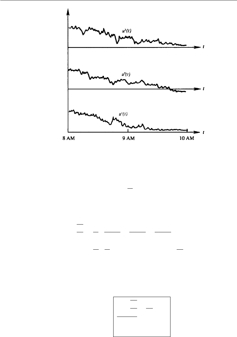
Figure 13.3 An ensemble of functions u(t).

each record and dividing the sum by the number of records. We therefore deﬁne the

ensemble average of u at time t to be

¯u(t) ≡



i=1

(t), (13.2)

where N is a large number. From this it follows that the average derivative at a certain

time is

∂u

∂t



∂u

(t)

∂t

∂u

(t)

∂t

∂u

(t)

∂t

+···



∂

∂t



(t) + u

(t) +···}



∂ ¯u

∂t

This shows that the operation of differentiation commutes with the operation of ensem-

ble averaging, so that their orders can be interchanged. In a similar manner we can

show that the operation of integration also commutes with ensemble averaging. We

therefore have the rules

∂u

∂t

∂ ¯u

∂t



udt =



¯udt.

(13.3)

(13.4)

4. Correlations and Spectra 543

Similar rules also hold when the variable is a function of space:

∂u

∂x

∂ ¯u

∂x

, (13.5)



udx =



¯udx. (13.6)

The rules of commutation (13.3)–(13.6) will be constantly used in the algebraic

manipulations throughout the chapter.

As there is no way of controlling natural phenomena in the atmosphere and the

ocean, it is very difﬁcult to obtain observations under identical conditions. Conse-

quently, in a nonstationary process such as the one shown in Figure 13.2b, the average

value of u at a certain time is sometimes determined by using equation (13.1) and

choosing an appropriate averaging time t

, small compared to the time during which

the average properties change appreciably. In any case, for theoretical discussions, all

averages deﬁned by overbars in this chapter are to be regarded as ensemble averages.

If the process also happens to be stationary, then the overbar can be taken to mean

the time average.

The various averages of a random variable, such as its mean and rms value,

are collectively called the statistics of the variable. When the statistics of a random

variable are independent of time, we say that the underlying process is stationary.

Examples of stationary and nonstationary processes are shown in Figure 13.2. For a

stationary process the time average (i.e., the average over a single record, deﬁned by

equation (13.1)) can be shown to equal the ensemble average, resulting in considerable

simpliﬁcation. Similarly, we deﬁne a homogeneous process as one whose statistics

are independent of space, for which the ensemble average equals the spatial average.

The mean square value of a variable is called the variance. The square root of

variance is called the root-mean-square (rms) value:

variance ≡

rms

≡ (u

)

1/2

The time series [u(t) −¯u], obtained after subtracting the mean ¯u of the series, repre-

sents the ﬂuctuation of the variable about its mean. The rms value of the ﬂuctuation

is called the standard deviation, deﬁned as

≡[(u −¯u)

]

1/2

4. Correlations and Spectra

The autocorrelation of a single variable u(t) at two times t

and t

is deﬁned as

R(t

) ≡ u(t

)u(t

). (13.7)

544 Turbulence

In the general case when the series is not stationary, the overbar is to be regarded

as an ensemble average. Then the correlation can be computed as follows: Obtain a

number of records of u(t), and on each record read off the values of u at t

and t

Then multiply the two values of u in each record and calculate the average value of

the product over the ensemble.

The magnitude of this average product is small when a positive value of u(t

) is

associated with both positive and negative values of u(t

). In such a case the magnitude

of R(t

) is small, and we say that the values of u at t

and t

are “weakly correlated.”

If, on the other hand, a positive value of u(t

) is mostly associated with a positive

value of u(t

), and a negative value of u(t

) is mostly associated with a negative value

of u(t

), then the magnitude of R(t

) is large and positive; in such a case we say

that the values of u(t

) and u(t

) are “strongly correlated.” We may also have a case

with R(t

) large and negative, in which one sign of u(t

) is mostly associated with

the opposite sign of u(t

For a stationary process the statistics (i.e., the various kinds of averages) are

independent of the origin of time, so that we can shift the origin of time by any

amount. Shifting the origin by t

, the autocorrelation (13.7) becomes u(0)u(t

− t

)

u(0)u(τ ), where τ = t

− t

is the time lag. It is clear that we can also write this

correlation as

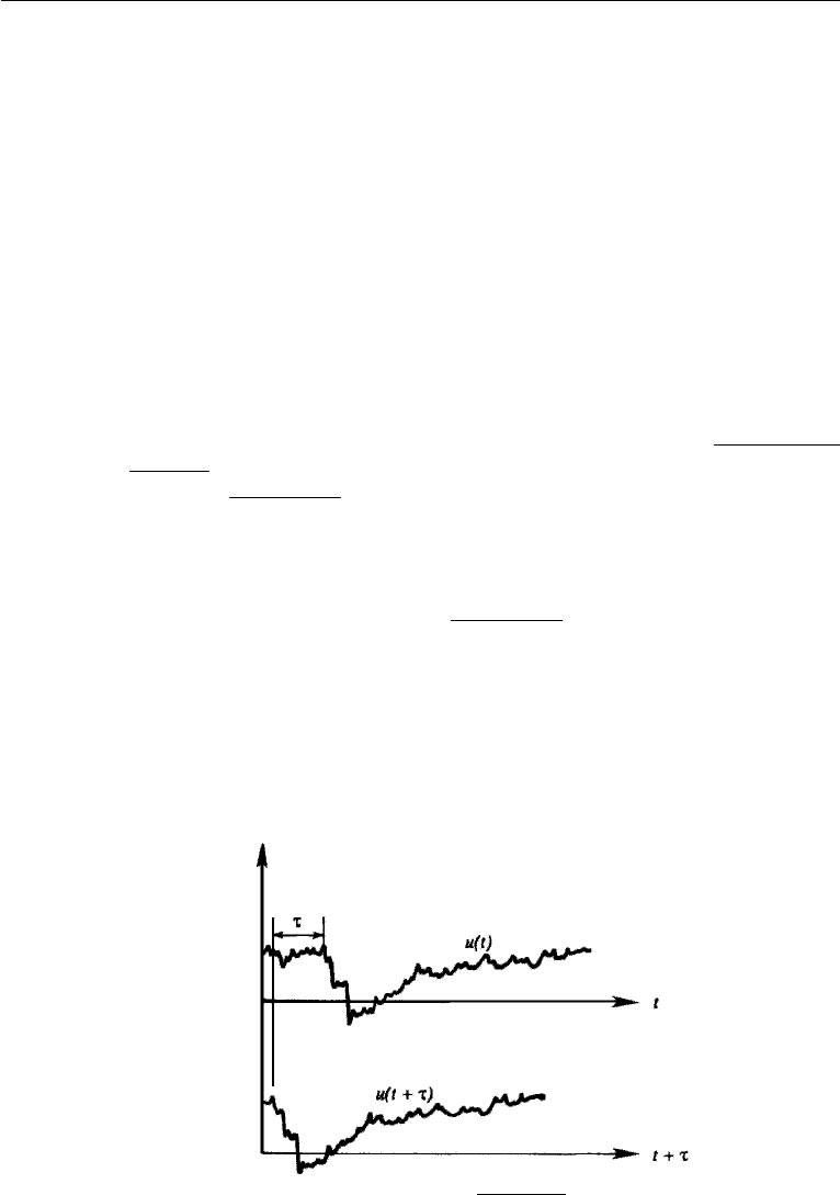
u(t)u(t +τ), which is a function of τ only, t being an arbitrary origin

of measurement. We can therefore deﬁne an autocorrelation function of a stationary

process by

R(τ) =

u(t)u(t +τ).

As we have assumed stationarity, the overbar in the aforementioned expression can

also be regarded as a time average. In such a case the method of estimating the

correlation is to align the series u(t) with u(t + τ) and multiply them vertically

(Figure 13.4).

Figure 13.4 Method of calculating autocorrelation u(t )u(t + τ).

4. Correlations and Spectra 545

We can also deﬁne a normalized autocorrelation function

r(τ) ≡

u(t)u(t +τ)

, (13.8)

where

is the mean square value. For any function u(t), it can be proved that

u(t

)u(t

)  [u

)]

1/2

)]

1/2

, (13.9)

which is called the Schwartz inequality. It is analogous to the rule that the inner product

of two vectors cannot be larger than the product of their magnitudes. For a stationary

process the mean square value is independent of time, so that the right-hand side of

equation (13.9) equals

. Using equation (13.9), it follows from equation (13.8) that

r  1.

Obviously, r(0) = 1. For a stationary process the autocorrelation is a symmetric

function, because then

R(τ) =

u(t)u(t +τ) = u(t −τ )u(t) = u(t)u(t − τ) = R(−τ).

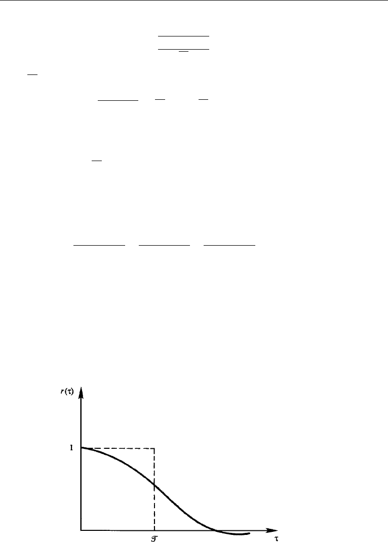
A typical autocorrelation plot is shown in Figure 13.5. Under normal conditions r goes

to0asτ →∞, because a process becomes uncorrelated with itself after a long time.

A measure of the width of the correlation function can be obtained by replacing

the measured autocorrelation distribution by a rectangle of height 1 and width

᐀

(Figure 13.5), which is therefore given by

᐀ ≡



∞

r(τ)dτ. (13.10)

Figure 13.5 Autocorrelation function and the integral time scale.

546 Turbulence

This is called the integral time scale, which is a measure of the time over which u(t)

is highly correlated with itself. In other words,

᐀ is a measure of the “memory” of

the process.

Let S(ω) denote the Fourier transform of the autocorrelation function R(τ).By

deﬁnition, this means that

S(ω) ≡

2π



∞

−∞

−iωτ

R(τ) dτ. (13.11)

It can be shown that, for equation (13.11) to be true, R(τ) must be given in terms of

S(ω) by

R(τ) ≡



∞

−∞

iωτ

S(ω) dω. (13.12)

We say that equations (13.11) and (13.12) deﬁne a “Fourier transform pair.” The

relationships (13.11) and (13.12) are not special for the autocorrelation function, but

hold for any function for which a Fourier transform can be deﬁned. Roughly speaking,

a Fourier transform can be deﬁned if the function decays to zero fast enough at inﬁnity.

It is easy to show that S(ω) is real and symmetric if R(τ) is real and symmetric

(Exercise 1). Substitution of τ = 0 in equation (13.12) gives



∞

−∞

S(ω) dω. (13.13)

This shows that S(ω)dω is the energy (more precisely, variance) in a frequency

band dω centered at ω. Therefore, the function S(ω) represents the way energy is

distributed as a function of frequency ω. We say that S(ω) is the energy spectrum, and

equation (13.11) shows that it is simply the Fourier transform of the autocorrelation

function. From equation (13.11) it also follows that

S(0) =

2π



∞

−∞

R(τ) dτ =



∞

r(τ)dτ =

᐀

which shows that the value of the spectrum at zero frequency is proportional to the

integral time scale.

So far we have considered u as a function of time and have deﬁned its autocor-

relation R(τ). In a similar manner we can deﬁne an autocorrelation as a function of

the spatial separation between measurements of the same variable at two points. Let

u(x

,t)and u(x

+x,t)denote the measurements of u at points x

and x

+x. Then

the spatial correlation is deﬁned as

u(x

, t)u(x

+ x,t). If the ﬁeld is spatially homo-

geneous, then the statistics are independent of the location x

, so that the correlation

depends only on the separation x :

R(x) =

u(x

, t)u(x

+ x,t).

5. Averaged Equations of Motion 547

We can now deﬁne an energy spectrum S(K) as a function of the wavenumber vector K

by the Fourier transform

S(K) =

(2π)

1/3



∞

−∞

−iK ·x

R(x)dx, (13.14)

where

R(x) =



∞

−∞

iK ·x

S(K)dK. (13.15)

The pair (13.14) and (13.15) is analogous to equations (13.11) and (13.12). In the

integral (13.14), dx is the shorthand notation for the volume element dx dy dz. Simi-

larly, in the integral (13.15), dK = dk dl dmis the volume element in the wavenumber

space (k,l,m).

It is clear that we need an instantaneous measurement u(x) as a function of

position to calculate the spatial correlations R(x). This is a difﬁcult task and so we

frequently determine this value approximately by rapidly moving a probe in a desired

direction. If the speed U

of traversing of the probe is rapid enough, we can assume

that the turbulence ﬁeld is “frozen” and does not change during the measurement.

Although the probe actually records a time series u(t), we may then transform it

to a spatial series u(x) by replacing t by x/U

. The assumption that the turbulent

ﬂuctuations at a point are caused by the advection of a frozen ﬁeld past the point is

called Taylor’s hypothesis.

So far we have deﬁned autocorrelations involving measurements of the same

variable u. We can also deﬁne a cross-correlation function between two stationary

variables u(t) and v(t) as

C(τ) ≡

u(t)v(t + τ).

Unlike the autocorrelation function, the cross-correlation function is not a symmetric

function of the time lag τ , because C(−τ) =

u(t)v(t − τ) = C(τ). The value of the

cross-correlation function at zero lag, that is

u(t)v(t ), is simply written as uv and

called the “correlation” of u and v.

5. Averaged Equations of Motion

A turbulent ﬂow instantaneously satisﬁes the Navier–Stokes equations. However, it

is virtually impossible to predict the ﬂow in detail, as there is an enormous range

of scales to be resolved, the smallest spatial scales being less than millimeters and

the smallest time scales being milliseconds. Even the most powerful of today’s com-

puters would take an enormous amount of computing time to predict the details of

an ordinary turbulent ﬂow, resolving all the ﬁne scales involved. Fortunately, we are

generally interested in ﬁnding only the gross characteristics in such a ﬂow, such as

the distributions of mean velocity and temperature. In this section we shall derive the

equations of motion for the mean state in a turbulent ﬂow and examine what effect

the turbulent ﬂuctuations may have on the mean ﬂow.

548 Turbulence

We assume that the density variations are caused by temperature ﬂuctuations

alone. The density variations due to other sources such as the concentration of a solute

can be handled within the present framework by deﬁning an equivalent temperature.

Under the Boussinesq approximation, the equations of motion for the instantaneous

variables are

∂ ˜u

∂t

+˜u

∂ ˜u

∂x

=−

∂ ˜p

∂x

− g[1 − α(

T − T

)]δ

+ ν

∂

˜u

∂x

, (13.16)

∂ ˜u

∂x

= 0, (13.17)

∂

∂t

+˜u

∂

∂x

= κ

∂

∂x

. (13.18)

As in the preceding chapter, we are denoting the instantaneous quantities by a

tilde ( ˜ ). Let the variables be decomposed into their mean part and a deviation from

the mean:

˜u

= U

+ u

˜p = P + p,

T =

T + T



(13.19)

(The corresponding density is ˜ρ =¯ρ +ρ



.) This is called the Reynolds decomposition.

As in the preceding chapter, the mean velocity and the mean pressure are denoted by

uppercase letters, and their turbulent ﬂuctuations are denoted by lowercase letters.

This convention is impossible to use for temperature and density, for which we use an

overbar for the mean state and a prime for the turbulent part. The mean quantities

(U, P ,

T)are to be regarded as ensemble averages; for stationary ﬂows they can also

be regarded as time averages. Taking the average of both sides of equation (13.19),

we obtain

¯u

=¯p = T



= 0,

showing that the ﬂuctuations have zero mean.

The equations satisﬁed by the mean ﬂow are obtained by substituting the

Reynolds decomposition (13.19) into the instantaneous Navier–Stokes equations

(13.16)–(13.18) and taking the average of the equations. The three equations transform

as follows.

Mean Continuity Equation

Averaging the continuity equation (13.17), we obtain

∂

∂x

+ u

) =

∂U

∂x

∂u

∂x

∂U

∂x

∂ ¯u

∂x

= 0,

5. Averaged Equations of Motion 549

where we have used the commutation rule (13.5). Using ¯u

= 0, we obtain

∂U

∂x

= 0, (13.20)

which is the continuity equation for the mean ﬂow. Subtracting this from the continuity

equation (13.17) for the total ﬂow, we obtain

∂u

∂x

= 0, (13.21)

which is the continuity equation for the turbulent ﬂuctuation ﬁeld. It is therefore seen

that the instantaneous, the mean, and the turbulent parts of the velocity ﬁeld are all

nondivergent.

Mean Momentum Equation

The momentum equation (13.16) gives

∂

∂t

+ u

) + (U

+ u

)

∂

∂x

+ u

)

=−

∂

∂x

(P + p) − g[1 − α(

T + T



− T

)]δ

+ ν

∂

∂x

+ u

). (13.22)

We shall take the average of each term of this equation. The average of the time

derivative term is

∂

∂t

+ u

) =

∂U

∂t

∂u

∂t

∂U

∂t

∂ ¯u

∂t

∂U

∂t

where we have used the commutation rule (13.3), and ¯u

= 0. The average of the

advective term is

+ u

)

∂

∂x

+ u

) = U

∂U

∂x

+ U

∂ ¯u

∂x

+¯u

∂U

∂x

+ u

∂u

∂x

= U

∂U

∂x

∂

∂x

where we have used the commutation rule (13.5) and ¯u

= 0; the continuity equation

∂u

/∂x

= 0 has also been used in obtaining the last term.

The average of the pressure gradient term is

∂

∂x

(P + p) =

∂P

∂x

∂ ¯p

∂x

∂P

∂x

550 Turbulence

The average of the gravity term is

[1 − α(

T + T



− T

)]=g[1 − α(

T − T

)],

where we have used



= 0. The average of the viscous term is

∂

∂x

+ u

) = ν

∂

∂x

Collecting terms, the mean of the momentum equation (13.22) takes the form

∂U

∂t

+ U

∂U

∂x

∂

∂x

) =−

∂P

∂x

− g[1 − α(

T − T

)]δ

+ ν

∂

∂x

(13.23)

The correlation

in equation (13.23) is generally nonzero, although ¯u

= 0. This

is discussed further in what follows.

Reynolds Stress

Writing the term

on the right-hand side, the mean momentum equation (13.23)

becomes

=−

∂P

∂x

− g[1 − α(

T − T

)]δ

∂

∂x



∂U

∂x

− u



, (13.24)

which can be written as

∂ ¯τ

∂x

− g[1 − α(

T − T

)]δ

(13.25)

where

¯τ

=−Pδ

+ µ



∂U

∂x

∂U

∂x



− ρ

. (13.26)

Compare equations (13.25) and (13.26) with the corresponding equations for the

instantaneous ﬂow, given by (see equations (4.13) and (4.36))

D ˜u

∂ ˜τ

∂x

− g[1 − α(

T − T

)]δ

˜τ

=−˜pδ

+ µ



∂ ˜u

∂x

∂ ˜u

∂x



It is seen from equation (13.25) that there is an additional stress −ρ

acting in a

mean turbulent ﬂow. In fact, these extra stresses on the mean ﬁeld of a turbulent ﬂow

5. Averaged Equations of Motion 551

are much larger than the viscous contribution µ(∂U

/∂x

+ ∂U

/∂x

), except very

close to a solid surface where the ﬂuctuations are small and mean ﬂow gradients are

large.

The tensor −ρ

is called the Reynolds stress tensor and has the nine Cartesian

components







−ρ

uv −ρ

−ρ

uv −ρ

−ρ

uw −ρ

vw −ρ







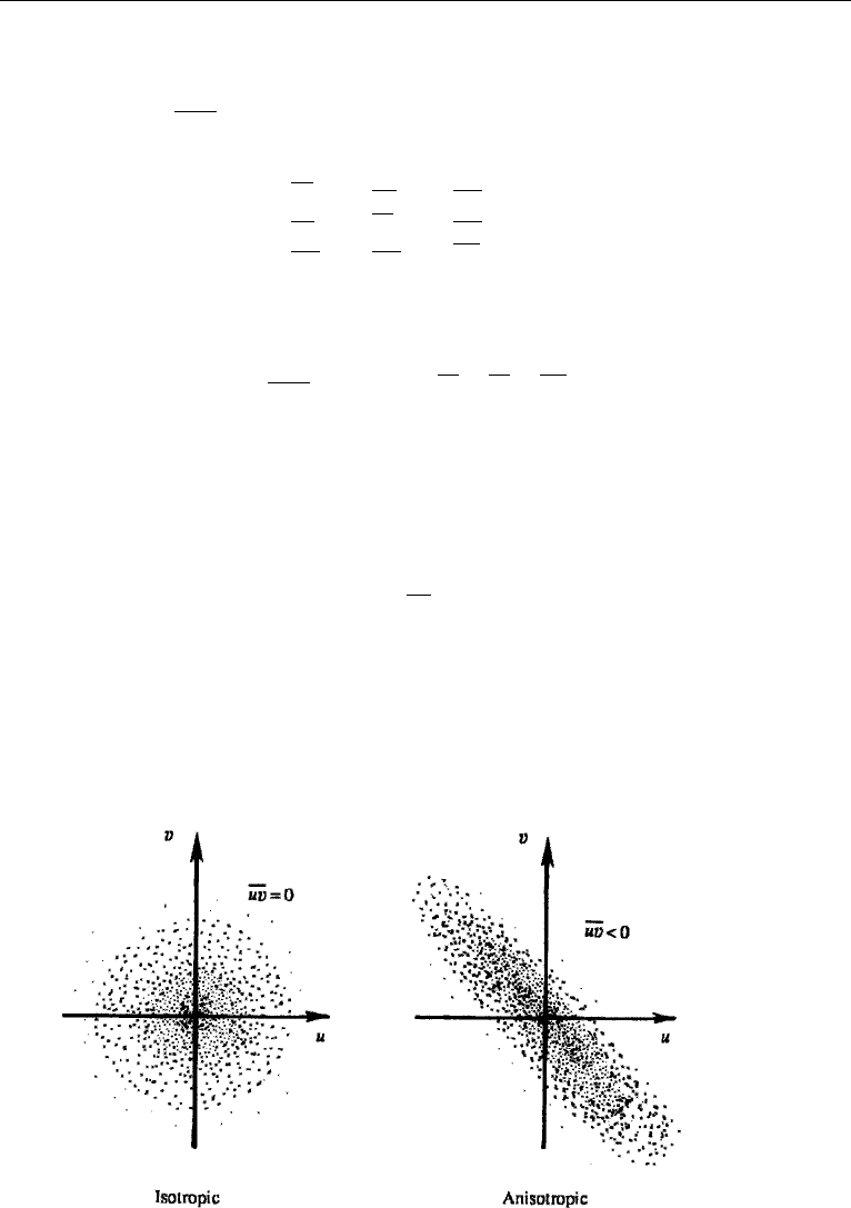
This is a symmetric tensor; its diagonal components are normal stresses, and the

off-diagonal components are shear stresses. If the turbulent ﬂuctuations are com-

pletely isotropic, that is, if they do not have any directional preference, then the

off-diagonal components of

vanish, and u

= v

= w

. This is shown in

Figure 13.6, which shows a cloud of data points (sometimes called a “scatter plot”)

on a uv-plane. The dots represent the instantaneous values of the uv-pair at different

times. In the isotropic case there is no directional preference, and the dots form a

spherically symmetric pattern. In this case a positive u is equally likely to be asso-

ciated with both a positive and a negative v. Consequently, the average value of the

product uv is zero if the turbulence is isotropic. In contrast, the scatter plot in an

anisotropic turbulent ﬁeld has a polarity. The ﬁgure shows a case where a positive u

is mostly associated with a negative v, giving

uv < 0.

It is easy to see why the average product of the velocity ﬂuctuations in a turbulent

ﬂow is not expected to be zero. Consider a shear ﬂow where the mean shear dU/dy

is positive (Figure 13.7). Assume that a particle at level y is instantaneously traveling

upward (v > 0). On the average the particle retains its original velocity during the

migration, and when it arrives at level y +dy it ﬁnds itself in a region where a larger

velocity prevails. Thus the particle tends to slow down the neighboring ﬂuid particles

Figure 13.6 Isotropic and anisotropic turbulent ﬁelds. Each dot represents a uv-pair at a certain time.