Cohen I.M., Kundu P.K. Fluid Mechanics

Подождите немного. Документ загружается.

522 Instability

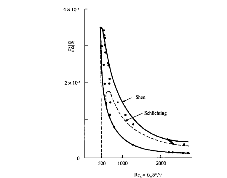
Figure 12.26 Marginal stability curve for a Blasius boundary layer. Theoretical solutions of Shen and

Schlichting are compared with experimental data of Schubauer and Skramstad.

Reshotko (2001) provides a review of temporally and spatially transient growth as

a path from subcritical (Tollmien–Schlichting) disturbances to transition. Growth or

decay is studied from the Orr–Sommerfeld and Squire equations. Growth may occur

because eigenfunctions of these equations are not orthogonal as the operators are not

self-adjoint. Results for Poiseuille pipe ﬂow and compressible blunt body ﬂows are

given.

Fransson and Alfredsson (2003) have shown that the asymptotic suction proﬁle

[solved in Exercise 9, Chapter 10] signiﬁcantly delays transition stimulated by free

stream turbulence or by Tollmien-Schlichting waves. Speciﬁcally, the value of Re

520 based on δ

∗

in Table 12.1 is increased for suction velocity ratio to v

∞

−.00288 over 54000. The very large stabilizing effect is a result of the change in

the shape of the streamwise velocity from the Blasius proﬁle to an exponential. The

normal suction velocity has a very small effect on stability.

12. Comments on Nonlinear Effects

To this point we have discussed only linear stability theory, which considers inﬁnites-

imal perturbations and predicts exponential growth when the relevant parameter

13. Transition 523

exceeds a critical value. The effect of the perturbations on the basic ﬁeld is neglected in

the linear theory. An examination of equation (12.83) shows that the perturbation ﬁeld

must be such that the mean Reynolds stress

uv (the “mean” being over a wavelength)

be nonzero for the perturbations to extract energy from the basic shear; similarly, the

heat ﬂux



must be nonzero in a thermal convection problem. These rectiﬁed ﬂuxes

of momentum and heat change the basic velocity and temperature ﬁelds. The linear

instability theory neglects these changes of the basic state. A consequence of the con-

stancy of the basic state is that the growth rate of the perturbations is also constant,

leading to an exponential growth. Within a short time of such initial growth the pertur-

bations become so large that the rectiﬁed ﬂuxes of momentum and heat signiﬁcantly

change the basic state, which in turn alters the growth of the perturbations.

A frequent effect of nonlinearity is to change the basic state in such a way as

to stop the growth of the disturbances after they have reached signiﬁcant amplitude

through the initial exponential growth. (Note, however, that the effect of nonlinearity

can sometimes be destabilizing; for example, the instability in a pipe ﬂow may be

a ﬁnite amplitude effect because the ﬂow is stable to inﬁnitesimal disturbances.)

Consider the thermal convection in the annular space between two vertical cylinders

rotating at the same speed. The outer wall of the annulus is heated and the inner wall

is cooled. For small heating rates the ﬂow is steady. For large heating rates a system of

regularly spaced waves develop and progress azimuthally at a uniform speed without

changing their shape. (This is the equilibrated form of baroclinic instability, discussed

in Chapter 14, Section 17.) At still larger heating rates an irregular, aperiodic, or

chaotic ﬂow develops. The chaotic response to constant forcing (in this case the

heating rate) is an interesting nonlinear effect and is discussed further in Section 14.

Meanwhile, a brief description of the transition from laminar to turbulent ﬂow is given

in the next section.

13. Transition

The process by which a laminar ﬂow changes to a turbulent one is called transition.

Instability of a laminar ﬂow does not immediately lead to turbulence, which is a

severely nonlinear and chaotic stage characterized by macroscopic “mixing” of ﬂuid

particles.After the initial breakdown of laminar ﬂow because of ampliﬁcation of small

disturbances, the ﬂow goes through a complex sequence of changes, ﬁnally resulting

in the chaotic state we call turbulence. The process of transition is greatly affected by

such experimental conditions as intensity of ﬂuctuations of the free stream, roughness

of the walls, and shape of the inlet. The sequence of events that lead to turbulence is

also greatly dependent on boundary geometry. For example, the scenario of transition

in a wall-bounded shear ﬂow is different from that in free shear ﬂows such as jets

and wakes.

Early stages of the transition consist of a succession of instabilities on increas-

ingly complex basic ﬂows, an idea ﬁrst suggested by Landau in 1944. The basic

state of wall-bounded parallel shear ﬂows becomes unstable to two-dimensional TS

waves, which grow and eventually reach equilibrium at some ﬁnite amplitude. This

steady state can be considered a new background state, and calculations show that

524 Instability

it is generally unstable to three-dimensional waves of short wavelength, which vary

in the “spanwise” direction. (If x is the direction of ﬂow and y is the directed nor-

mal to the boundary, then the z-axis is spanwise.) We shall call this the secondary

instability. Interestingly, the secondary instability does not reach equilibrium at ﬁnite

amplitude but directly evolves to a fully turbulent ﬂow. Recent calculations of the

secondary instability have been quite successful in reproducing critical Reynolds

numbers for various wall-bounded ﬂows, as well as predicting three-dimensional

structures observed in experiments.

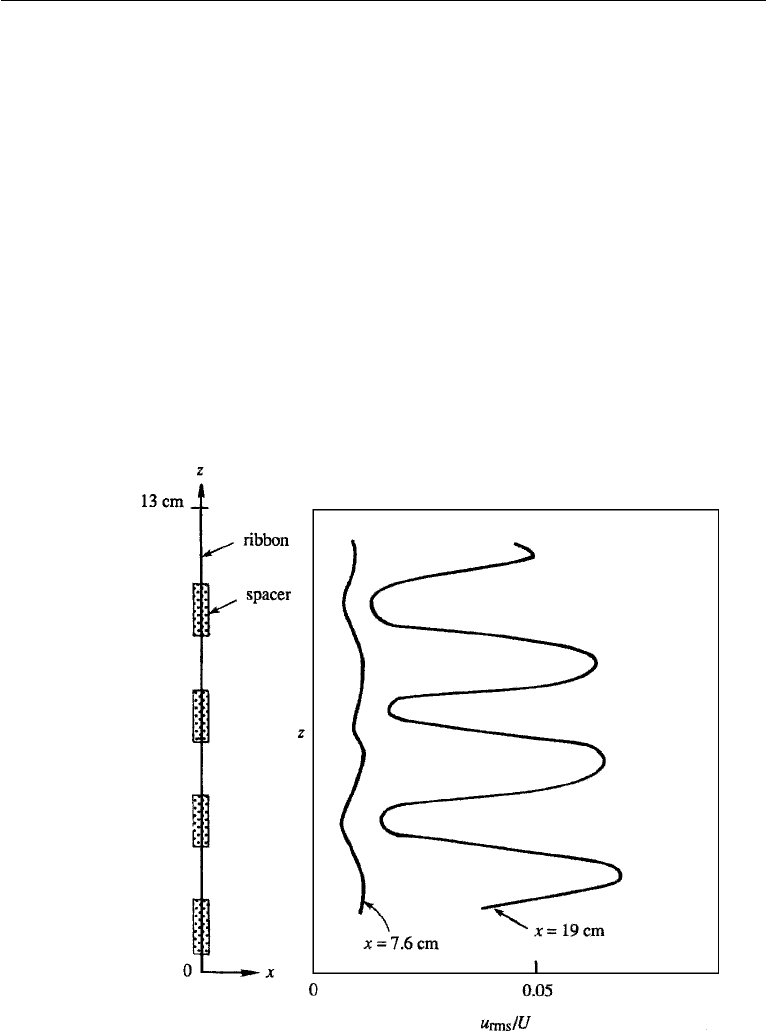
A key experiment on the three-dimensional nature of the transition process in a

boundary layer was performed by Klebanoff, Tidstrom, and Sargent (1962). They con-

ducted a series of controlled experiments by which they introduced three-dimensional

disturbances on a ﬁeld of TS waves in a boundary layer. The TS waves were as usual

artiﬁcially generated by an electromagnetically vibrated ribbon, and the three dimen-

sionality of a particular spanwise wavelength was introduced by placing spacers

(small pieces of transparent tape) at equal intervals underneath the vibrating ribbon

(Figure 12.27). When the amplitude of the TS waves became roughly 1% of the

free-stream velocity, the three-dimensional perturbations grew rapidly and resulted

Figure 12.27 Three-dimensional unstable waves initiated by vibrating ribbon. Measured distributions of

intensity of the u-ﬂuctuation at two distances from the ribbon are shown. P. S. Klebanoff et al., Journal of

Fluid Mechanics 12: 1–34, 1962 and reprinted with the permission of Cambridge University Press.

14. Deterministic Chaos 525

in a spanwise irregularity of the streamwise velocity displaying peaks and valleys

in the amplitude of u. The three-dimensional disturbances continued to grow until

the boundary layer became fully turbulent. The chaotic ﬂow seems to result from the

nonlinear evolution of the secondary instability, and recent numerical calculations

have accurately reproduced several characteristic features of real ﬂows (see Figures 7

and 8 in Bayly et al., 1988).

It is interesting to compare the chaos observed in turbulent shear ﬂows with

that in controlled low-order dynamical systems such as the B´ernard convection or

Taylor vortex ﬂow. In these low-order ﬂows only a very small number of modes

participate in the dynamics because of the strong constraint of the boundary con-

ditions. All but a few low modes are identically zero, and the chaos develops in

an orderly way. As the constraints are relaxed (we can think of this as increas-

ing the number of allowed Fourier modes), the evolution of chaos becomes less

orderly.

Transition in a free shear layer, such as a jet or a wake, occurs in a different manner.

Because of the inﬂectional velocity proﬁles involved, these ﬂows are unstable at a very

low Reynolds numbers, that is, of order 10 compared to about 10

for a wall-bounded

ﬂow. The breakdown of the laminar ﬂow therefore occurs quite readily and close

to the origin of such a ﬂow. Transition in a free shear layer is characterized by the

appearance of a rolled-up row of vortices, whose wavelength corresponds to the one

with the largest growth rate. Frequently, these vortices group themselves in the form

of pairs and result in a dominant wavelength twice that of the original wavelength.

Small-scale turbulence develops within these larger scale vortices, ﬁnally leading to

turbulence.

14. Deterministic Chaos

The discussion in the previous section has shown that dissipative nonlinear systems

such as ﬂuid ﬂows reach a random or chaotic state when the parameter measuring

nonlinearity (say, the Reynolds number or the Rayleigh number) is large. The change

to the chaotic stage generally takes place through a sequence of transitions, with the

exact route depending on the system. It has been realized that chaotic behavior not only

occurs in continuous systems having an inﬁnite number of degrees of freedom, but

also in discrete nonlinear systems having only a small number of degrees of freedom,

governed by ordinary nonlinear differential equations. In this context, a chaotic system

is deﬁned as one in which the solution is extremely sensitive to initial conditions. That

is, solutions with arbitrarily close initial conditions evolve into quite different states.

Other symptoms of a chaotic system are that the solutions are aperiodic, and that the

spectrum is broadband instead of being composed of a few discrete lines.

Numerical integrations (to be shown later in this section) have recently demon-

strated that nonlinear systems governed by a ﬁnite set of deterministic ordinary dif-

ferential equations allow chaotic solutions in response to a steady forcing. This fact is

interesting because in a dissipative linear system a constant forcing ultimately (after

the decay of the transients) leads to constant response, a periodic forcing leads to

periodic response, and a random forcing leads to random response. In the presence

526 Instability

of nonlinearity, however, a constant forcing can lead to a variable response, both

periodic and aperiodic. Consider again the experiment mentioned in Section 12,

namely, the thermal convection in the annular space between two vertical cylinders

rotating at the same speed. The outer wall of the annulus is heated and the inner wall

is cooled. For small heating rates the ﬂow is steady. For large heating rates a system

of regularly spaced waves develops and progresses azimuthally at a uniform speed,

without the waves changing shape. At still larger heating rates an irregular, aperiodic,

or chaotic ﬂow develops. This experiment shows that both periodic and aperiodic ﬂow

can result in a nonlinear system even when the forcing (in this case the heating rate)

is constant. Another example is the periodic oscillation in the ﬂow behind a blunt

body at Re ∼ 40 (associated with the initial appearance of the von Karman vortex

street) and the breakdown of the oscillation into turbulent ﬂow at larger values of the

Reynolds number.

It has been found that transition to chaos in the solution of ordinary nonlinear

differential equations displays a certain universal behavior and proceeds in one of a

few different ways. At the moment it is unclear whether the transition in ﬂuid ﬂows is

closely related to the development of chaos in the solutions of these simple systems;

this is under intense study. In this section we shall discuss some of the elementary

ideas involved, starting with certain deﬁnitions. An introduction to the subject of

chaos is given by Berg´e, Pomeau, and Vidal (1984); a useful review is given in

Lanford (1982). The subject has far-reaching cosmic consequences in physics and

evolutionary biology, as discussed by Davies (1988).

Phase Space

Very few nonlinear equations have analytical solutions. For nonlinear systems, a

typical procedure is to ﬁnd a numerical solution and display its properties in a space

whose axes are the dependent variables. Consider the equation governing the motion

of a simple pendulum of length l:

X +

sin X = 0,

where X is the angular displacement and

X(= d

X/dt

) is the angular acceleration.

(The component of gravity parallel to the trajectory is −g sin X, which is balanced by

the linear acceleration l

X.) The equation is nonlinear because of the sin X term. The

second-order equation can be split into two coupled ﬁrst-order equations

X = Y,

Y =−

sin X.

(12.84)

Starting with some initial conditions on X and Y , one can integrate set (12.84). The

behavior of the system can be studied by describing how the variables Y (=

X) and X

vary as a function of time. For the pendulum problem, the space whose axes are

X and

X is called a phase space, and the evolution of the system is described by a trajectory

14. Deterministic Chaos 527

in this space. The dimension of the phase space is called the degree of freedom of the

system; it equals the number of independent initial conditions necessary to specify

the system. For example, the degree of freedom for the set (12.84) is two.

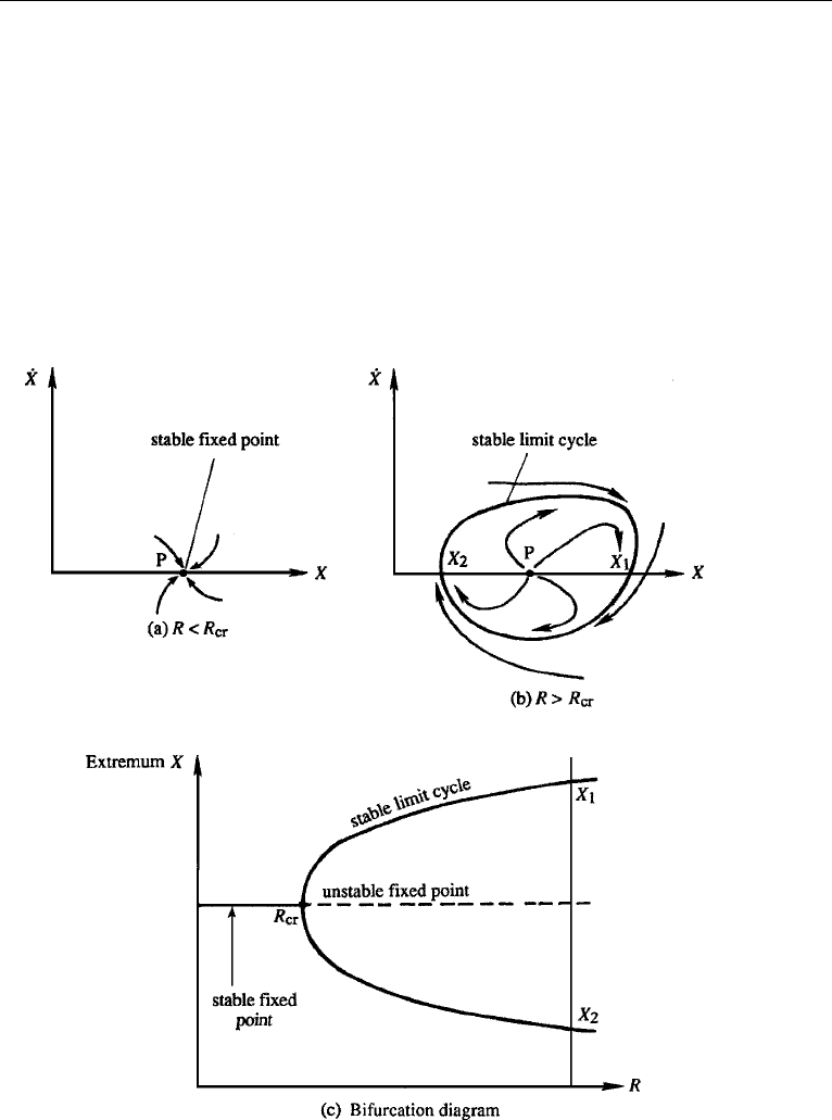
Attractor

Dissipative systems are characterized by the existence of attractors, which are struc-

tures in the phase space toward which neighboring trajectories approach as t →∞.

An attractor can be a ﬁxed point representing a stable steady ﬂow or a closed

curve (called a limit cycle) representing a stable oscillation (Figure 12.28a, b). The

nature of the attractor depends on the value of the nonlinearity parameter, which

Figure 12.28 Attractors in a phase plane. In (a), point P is an attractor. For a larger value of R, panel

(b) shows that P becomes an unstable ﬁxed point (a “repeller”), and the trajectories are attracted to a limit

cycle. Panel (c) is the bifurcation diagram.

528 Instability

will be denoted by R in this section. As R is increased, the ﬁxed point represent-

ing a steady solution may change from being an attractor to a repeller with spi-

rally outgoing trajectories, signifying that the steady ﬂow has become unstable to

inﬁnitesimal perturbations. Frequently, the trajectories are then attracted by a limit

cycle, which means that the unstable steady solution gives way to a steady oscil-

lation (Figure 12.28b). For example, the steady ﬂow behind a blunt body becomes

oscillatory as Re is increased, resulting in the periodic von Karman vortex street

(Figure 10.18).

The branching of a solution at a critical value R

of the nonlinearity parameter

is called a bifurcation. Thus, we say that the stable steady solution of Figure 12.28a

bifurcates to a stable limit cycle as R increases through R

. This can be represented

on the graph of a dependent variable (say, X)vsR (Figure 12.28c). At R = R

, the

solution curve branches into two paths; the two values of X on these branches (say,

and X

) correspond to the maximum and minimum values of X in Figure 12.28b.

It is seen that the size of the limit cycle grows larger as (R − R

) becomes larger.

Limit cycles, representing oscillatory response with amplitude independent of initial

conditions, are characteristic features of nonlinear systems. Linear stability theory

predicts an exponential growth of the perturbations if R>R

, but a nonlinear theory

frequently shows that the perturbations eventually equilibrate to a steady oscillation

whose amplitude increases with (R − R

The Lorenz Model of Thermal Convection

Taking the example of thermal convection in a layer heated from below (the B´enard

problem), Lorenz (1963) demonstrated that the development of chaos is associated

with the attractor acquiring certain strange properties. He considered a layer with

stress-free boundaries. Assuming nonlinear disturbances in the form of rolls invariant

in the y direction, and deﬁning a streamfunction in the xz-plane by u =−∂ψ/∂z and

w = ∂ψ/∂x, he substituted solutions of the form

ψ ∝ X(t) cos πzsin kx,



∝ Y(t)cos πzcos kx + Z(t) sin 2πz,

(12.85)

into the equations of motion (12.7). Here, T



is the departure of temperature from the

state of no convection, k is the wavenumber of the perturbation, and the boundaries

are at z =±

. It is clear that X is proportional to the intensity of convective motion, Y

is proportional to the temperature difference between the ascending and descending

currents, and Z is proportional to the distortion of the average vertical proﬁle of

temperature from linearity. (Note in equation (12.85) that the x-average of the term

multiplied by Y(t) is zero, so that this term does not cause distortion of the basic

temperature proﬁle.) As discussed in Section 3, Rayleigh’s linear analysis showed that

solutions of the form (12.85), with X and Y constants and Z = 0, would develop if Ra

slightly exceeds the critical value Ra

= 27 π

/4. Equations (12.85) are expected to

give realistic results when Ra is slightly supercritical but not when strong convection

occurs because only the lowest terms in a “Galerkin expansion” are retained.

14. Deterministic Chaos 529

On substitution of equation (12.85) into the equations of motion, Lorenz ﬁnally

obtained

X = Pr(Y − X),

Y =−XZ + rX − Y,

Z = XY − bZ,

(12.86)

where Pr is the Prandtl number, r = Ra/Ra

, and b = 4π

/(π

+ k

). Equations

(12.86) represent a set of nonlinear equations with three degrees of freedom, which

means that the phase space is three-dimensional.

Equations (12.86) allow the steady solution X = Y = Z = 0, representing the

state of no convection. For r>1 the system possesses two additional steady-state

solutions, which we shall denote by

X =

Y =±

√

b(r − 1),

Z = r −1; the two signs

correspond to the two possible senses of rotation of the rolls. (The fact that these steady

solutions satisfy equation (12.86) can easily be checked by substitution and setting

X =

Y =

Z = 0.) Lorenz showed that the steady-state convection becomes unstable

if r is large. Choosing Pr = 10, b = 8/3, and r = 28, he numerically integrated the

set and found that the solution never repeats itself; it is aperiodic and wanders about

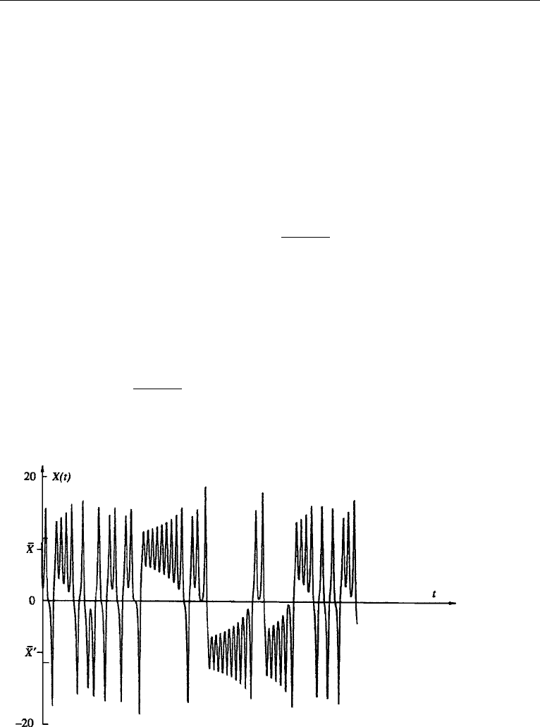
in a chaotic manner. Figure 12.29 shows the variation of X(t), starting with some

initial conditions. (The variables Y(t) and Z(t) also behave in a similar way.) It is

seen that the amplitude of the convecting motion initially oscillates around one of the

steady values

X =±

√

b(r − 1), with the oscillations growing in magnitude. When

it is large enough, the amplitude suddenly goes through zero to start oscillations of

opposite sign about the other value of

X. That is, the motion switches in a chaotic

Figure 12.29 Variation of X(t) in the Lorenz model. Note that the solution oscillates erratically around

the two steady values

X and



. P. Berg´e,Y. Pomeau, and C.Vidal, Order Within Chaus, 1984 and reprinting

permitted by Heinemann Educational, a division of Reed Educational & Professional Publishing Ltd.

530 Instability

manner between two oscillatory limit cycles, with the number of oscillations between

transitions seemingly random. Calculations show that the variables X, Y , and Z have

continuous spectra and that the solution is extremely sensitive to initial conditions.

Strange Attractors

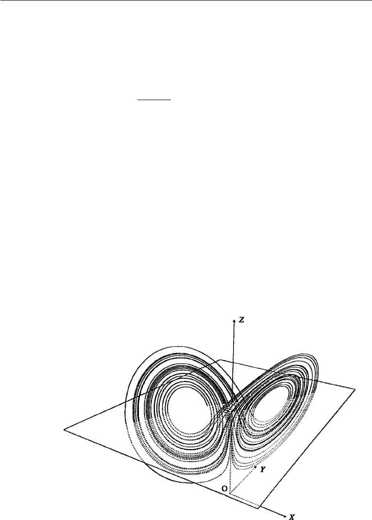
The trajectories in the phase plane in the Lorenz model of thermal convection are

shown in Figure 12.30. The centers of the two loops represent the two steady con-

vections

X =

Y =±

√

b(r − 1),

Z = r − 1. The structure resembles two rather ﬂat

loops of ribbon, one lying slightly in front of the other along a central band with the

two joined together at the bottom of that band. The trajectories go clockwise around

the left loop and counterclockwise around the right loop; two trajectories never inter-

sect. The structure shown in Figure 12.30 is an attractor because orbits starting with

initial conditions outside of the attractor merge on it and then follow it. The attraction

is a result of dissipation in the system. The aperiodic attractor, however, is unlike the

normal attractor in the form of a ﬁxed point (representing steady motion) or a closed

curve (representing a limit cycle). This is because two trajectories on the aperiodic

attractor, with inﬁnitesimally different initial conditions, follow each other closely

only for a while, eventually diverging to very different ﬁnal states. This is the basic

reason for sensitivity to initial conditions.

For these reasons the aperiodic attractor is called a strange attractor. The idea of

a strange attractor is quite nonintuitive because it has the dual property of attraction

and divergence. Trajectories are attracted from the neighboring region of phase space,

but once on the attractor the trajectories eventually diverge and result in chaos. An

ordinary attractor “forgets” slightly different initial conditions, whereas the strange

Figure 12.30 The Lorenz attractor. Centers of the two loops represent the two steady solutions (

Z).

14. Deterministic Chaos 531

attractor ultimately accentuates them. The idea of the strange attractor was ﬁrst

conceived by Lorenz, and since then attractors of other chaotic systems have also

been studied. They all have the common property of aperiodicity, continuous spectra,

and sensitivity to initial conditions.

Scenarios for Transition to Chaos

Thus far we have studied discrete dynamical systems having only a small number

of degrees of freedom and seen that aperiodic or chaotic solutions result when the

nonlinearity parameter is large. Several routes or scenarios of transition to chaos in

such systems have been identiﬁed. Two of these are described brieﬂy here.

(1) Transition through subharmonic cascade:AsR is increased, a typical non-

linear system develops a limit cycle of a certain frequency ω. With further

increase of R, several systems are found to generate additional frequencies

ω/2, ω/4, ω/8,.... The addition of frequencies in the form of subhar-

monics does not change the periodic nature of the solution, but the period

doubles each time a lower harmonic is added. The period doubling takes

place more and more rapidly as R is increased, until an accumulation point

(Figure 12.31) is reached, beyond which the solution wanders about in a chaotic

manner. At this point the peaks disappear from the spectrum, which becomes

continuous. Many systems approach chaotic behavior through period doubling.

Feigenbaum (1980) proved the important result that this kind of transition

develops in a universal way, independent of the particular nonlinear systems

studied. If R

represents the value for development of a new subharmonic,

then R

converges in a geometric series with

− R

n−1

n+1

− R

→ 4.6692 as n →∞.

That is, the horizontal gap between two bifurcation points is about a ﬁfth of the

previous gap. The vertical gap between the branches of the bifurcation diagram

also decreases, with each gap about two-ﬁfths of the previous gap. In other

words, the bifurcation diagram (Figure 12.31) becomes “self similar” as the

accumulation point is approached. (Note that Figure 12.31 has not been drawn

to scale, for illustrative purposes.) Experiments in low Prandtl number ﬂuids

(such as liquid metals) indicate that B´enard convection in the form of rolls

develops oscillatory motion of a certain frequency ω at Ra = 2Ra

.AsRais

further increased, additional frequencies ω/2, ω/4, ω/8, ω/16, and ω/32 have

been observed. The convergence ratio has been measured to be 4.4, close to the

value of 4.669 predicted by Feigenbaum’s theory. The experimental evidence

is discussed further in Berg´e, Pomeau, and Vidal (1984).

(2) Transition through quasi-periodic regime: Ruelle and Takens (1971) have

mathematically proved that certain systems need only a small number of

bifurcations to produce chaotic solutions. As the nonlinearity parameter is

increased, the steady solution loses stability and bifurcates to an oscillatory