Cohen I.M., Kundu P.K. Fluid Mechanics
Подождите немного. Документ загружается.

512 Instability
flows. He showed that a necessary condition for instability of inviscid parallel flows
is that U
yy
(U − U
I
)<0 somewhere in the flow, where U
I
is the value of U at the
point of inflection. To prove the theorem, take the real part of equation (12.78):
U
yy
(U − c
r
)
|U − c|
2
|φ|
2
dy =−
[|φ
y
|
2
+ k
2
|φ|
2
]dy < 0. (12.80)
Suppose that the flow is unstable, so that c
i
= 0, and a point of inflection does exist
according to the Rayleigh criterion. Then it follows from equation (12.79) that
(c
r
− U
I
)
U
yy
|φ|
2
|U − c|
2
dy = 0. (12.81)
Adding equations (12.80) and (12.81), we obtain
U
yy
(U − U
I
)
|U − c|
2
|φ|
2
dy < 0,
so that U
yy
(U − U
I
) must be negative somewhere in the flow.
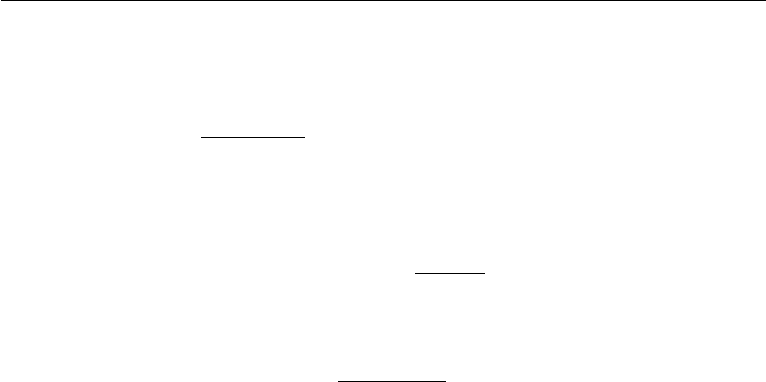
Some common velocity profiles are shown in Figure 12.21. Only the two flows
shown in the bottom row can possibly be unstable, for only they satisfy Fjortoft’s
theorem. Flows (a), (b), and (c) do not have any inflection point: flow (d) does satisfy
Rayleigh’s condition but not Fjortoft’s because U
yy
(U − U
I
) is positive. Note that
an alternate way of stating Fjortoft’s theorem is that the magnitude of vorticity of the
basic flow must have a maximum within the region of flow, not at the boundary. In
flow (d), the maximum magnitude of vorticity occurs at the walls.
The criteria of Rayleigh and Fjortoft essentially point to the importance of having
a point of inflection in the velocity profile. They show that flows in jets, wakes, shear
layers, and boundary layers with adverse pressure gradients, all of which have a point
of inflection and satisfy Fjortoft’s theorem, are potentially unstable. On the other
hand, plane Couette flow, Poiseuille flow, and a boundary layer flow with zero or
favorable pressure gradient have no point of inflection in the velocity profile, and are
stable in the inviscid limit.
However, neither of the two conditions is sufficient for instability. An example
is the sinusoidal profile U = sin y, with boundaries at y =±b. It has been shown
that the flow is stable if the width is restricted to 2b<π, although it has an inflection
point at y = 0.
Critical Layers
Inviscid parallel flows satisfy Howard’s semicircle theorem, which was proved in
Section 7 for the more general case of a stratified shear flow. The theorem states that
the phase speed c
r
has a value that lies between the minimum and the maximum
values of U(y) in the flow field. Now growing and decaying modes are characterized
by a nonzero c
i
, whereas neutral modes can have only a real c = c
r
. It follows that
neutral modes must have U = c somewhere in the flow field. The neighborhood y
around y
c
at which U = c = c
r
is called a critical layer. The point y
c
is a critical
9. Inviscid Stability of Parallel Flows 513
Figure 12.21 Examples of parallel flows. Points of inflection are denoted by I. Only (e) and (f) satisfy
Fjortoft’s criterion of inviscid instability.
point of the inviscid governing equation (12.76), because the highest derivative drops
out at this value of y. The solution of the eigenfunction is discontinuous across this
layer. The full Orr–Sommerfeld equation (12.74) has no such critical layer because
the highest-order derivative does not drop out when U = c. It is apparent that in a
real flow a viscous boundary layer must form at the location where U = c, and the
layer becomes thinner as Re →∞.
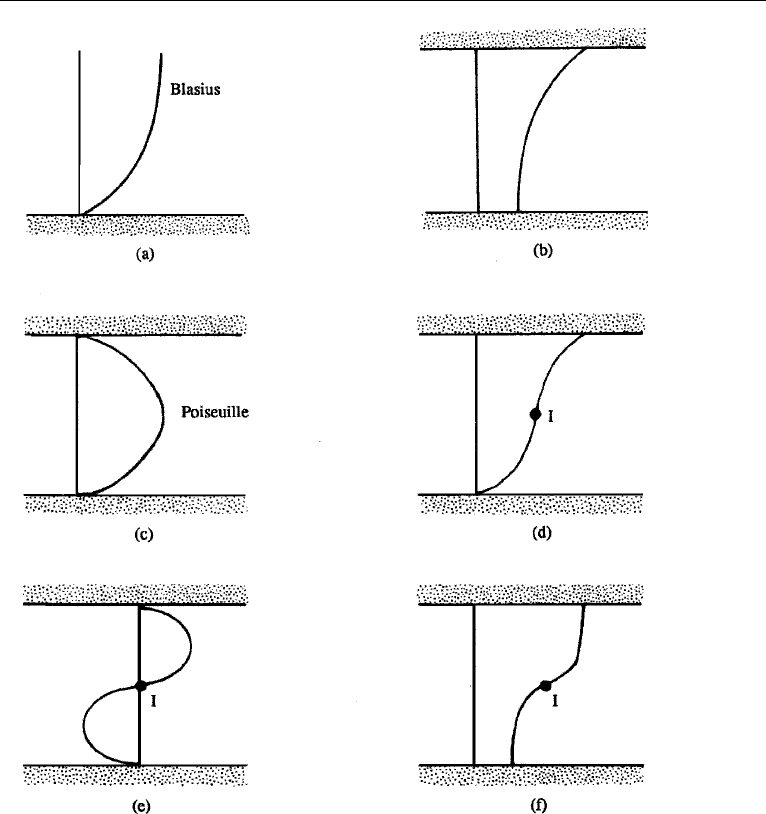
The streamline pattern in the neighborhood of the critical layer where U = c was
given by Kelvin in 1888; our discussion here is adapted from Drazin and Reid (1981).
514 Instability
Figure 12.22 The Kelvin cat’s eye pattern near a critical layer, showing streamlines as seen by an observer
moving with the wave.
Consider a flow viewed by an observer moving with the phase velocity c = c
r
. Then
the basic velocity field seen by this observer is (U − c), so that the streamfunction
due to the basic flow is
=
(U − c) dy.
The total streamfunction is obtained by adding the perturbation:
˜
ψ =
(U − c) dy + Aφ(y)e
ikx
, (12.82)
where A is an arbitrary constant, and we have omitted the time factor on the second
term because we are considering only neutral disturbances. Near the critical layer
y = y
c
, a Taylor series expansion shows that equation (12.82) is approximately
˜
ψ =
1
2
U
yc
(y − y
c
)
2
+ Aφ (y
c
) cos kx,
where U
yc
is the value of U
y
at y
c
; we have taken the real part of the right-hand side,
and taken φ(y
c
) to be real. The streamline pattern corresponding to the preceding
equation is sketched in Figure 12.22, showing the so-called Kelvin cat’s eye pattern.
10. Some Results of Parallel Viscous Flows
Our intuitive expectation is that viscous effects are stabilizing. The thermal and cen-
trifugal convections discussed earlier in this chapter have confirmed this intuitive
expectation. However, the conclusion that the effect of viscosity is stabilizing is not
always true. Consider the Poiseuille flow and the Blasius boundary layer profiles in
Figure 12.21, which do not have any inflection point and are therefore inviscidly
stable. These flows are known to undergo transition to turbulence at some Reynolds
number, which suggests that inclusion of viscous effects may in fact be destabiliz-
ing in these flows. Fluid viscosity may thus have a dual effect in the sense that it
can be stabilizing as well as destabilizing. This is indeed true as shown by stability
calculations of parallel viscous flows.
10. Some Results of Parallel Viscous Flows 515
The analytical solution of the Orr–Sommerfeld equation is notoriously
complicated and will not be presented here. The viscous term in (12.74) contains
the highest-order derivative, and therefore the eigenfunction may contain regions of
rapid variation in which the viscous effects become important. Sophisticated asymp-
totic techniques are therefore needed to treat these boundary layers. Alternatively,
solutions can be obtained numerically. For our purposes, we shall discuss only cer-
tain features of these calculations. Additional information can be found in Drazin and
Reid (1981), and in the review article by Bayly, Orszag, and Herbert (1988).
Mixing Layer
Consider a mixing layer with the velocity profile
U = U
0
tanh
y
L
.
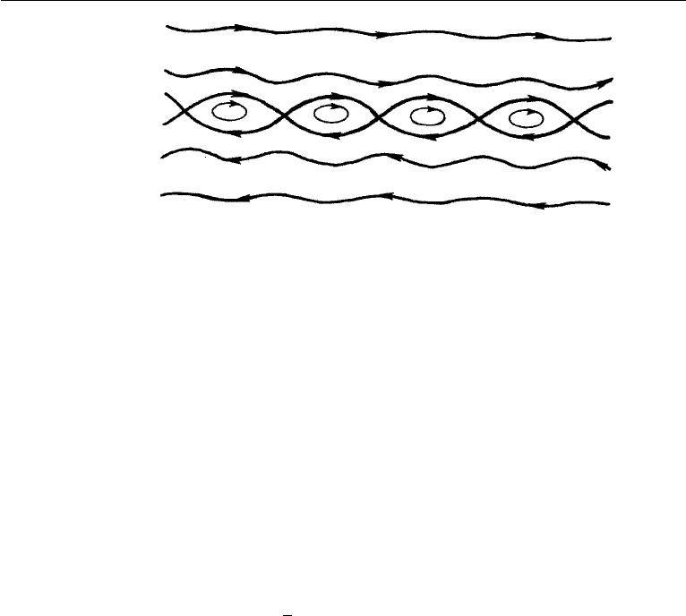
A stability diagram for solution of the Orr–Sommerfeld equation for this velocity
distribution is sketched in Figure 12.23. It is seen that at all Reynolds numbers the
flow is unstable to waves having low wavenumbers in the range 0 <k<k
u
, where
the upper limit k
u
depends on the Reynolds number Re = U
0
L/ν. For high values of
Re, the range of unstable wavenumbers increases to 0 <k<1/L, which corresponds
to a wavelength range of ∞ >λ>2πL. It is therefore essentially a long wavelength
instability.
Figure 12.23 implies that the critical Reynolds number in a mixing layer is zero. In
fact, viscous calculations for all flows with “inflectional profiles” show a small critical
Reynolds number; for example, for a jet of the form u = U sech
2
( y/L),itisRe
cr
= 4.
These wall-free shear flows therefore become unstable very quickly, and the inviscid
criterion that these flows are always unstable is a fairly good description. The reason
the inviscid analysis works well in describing the stability characteristics of free shear
Figure 12.23 Marginal stability curve for a shear layer u = U
0
tanh( y/L).

516 Instability
flows can be explained as follows. For flows with inflection points the eigenfunction
of the inviscid solution is smooth. On this zero-order approximation, the viscous
term acts as a regular perturbation, and the resulting correction to the eigenfunction
and eigenvalues can be computed as a perturbation expansion in powers of the small
parameter 1/Re. This is true even though the viscous term in the Orr–Sommerfeld
equation contains the highest-order derivative.
The instability in flows with inflection points is observed to form rolled-up blobs
of vorticity, much like in the calculations of Figure 12.18 or in the photograph of
Figure 12.16. This behavior is robust and insensitive to the detailed experimental
conditions. They are therefore easily observed. In contrast, the unstable waves in a
wall-bounded shear flow are extremely difficult to observe, as discussed in the next
section.
Plane Poiseuille Flow
The flow in a channel with parabolic velocity distribution has no point of inflection and
is inviscidly stable. However, linear viscous calculations show that the flow becomes
unstable at a critical Reynolds number of 5780. Nonlinear calculations, which con-
sider the distortion of the basic profile by the finite amplitude of the perturbations,
give a critical number of 2510, which agrees better with the observed transition.
In any case, the interesting point is that viscosity is destabilizing for this flow. The
solution of the Orr–Sommerfeld equation for the Poiseuille flow and other parallel
flows with rigid boundaries, which do not have an inflection point, is complicated.
In contrast to flows with inflection points, the viscosity here acts as a singular per-
turbation, and the eigenfunction has viscous boundary layers on the channel walls
and around critical layers where U = c
r
. The waves that cause instability in these
flows are called Tollmien–Schlichting waves, and their experimental detection is dis-
cussed in the next section. In his text, C. S. Yih gives a thorough discussion of the
solution of the Orr-Sommerfeld equation using asymptotic expansions in the limit
sequence Re →∞, then k → 0(butkRe 1). He follows closely the analysis
of W. Heisenberg (1924). Yih presents C. C. Lin’s improvements on Heisenberg’s
analysis with S. F. Shen’s calculations of the stability curves.
Plane Couette Flow
This is the flow confined between two parallel plates; it is driven by the motion of
one of the plates parallel to itself. The basic velocity profile is linear, with U = y.
Contrary to the experimentally observed fact that the flow does become turbulent
at high values of Re, all linear analyses have shown that the flow is stable to small
disturbances. It is now believed that the instability is caused by disturbances of finite
magnitude.
Pipe Flow
The absence of an inflection point in the velocity profile signifies that the flow is
inviscidly stable. All linear stability calculations of the viscous problem have also
shown that the flow is stable to small disturbances. In contrast, most experiments

10. Some Results of Parallel Viscous Flows 517
show that the transition to turbulence takes place at a Reynolds number of about
Re = U
max
d/ν ∼ 3000. However, careful experiments, some of them performed
by Reynolds in his classic investigation of the onset of turbulence, have been able to
maintain laminar flow until Re = 50,000. Beyond this the observed flow is invari-
ably turbulent. The observed transition has been attributed to one of the following
effects: (1) It could be a finite amplitude effect; (2) the turbulence may be initiated at
the entrance of the tube by boundary layer instability (Figure 9.2); and (3) the insta-
bility could be caused by a slow rotation of the inlet flow which, when added to the
Poiseuille distribution, has been shown to result in instability. This is still under inves-
tigation. New insights into the instability and transition of pipe flow were described by
Eckhardt et al. (2007) by analysis via dynamical systems theory and comparison with
recent very carefully crafted experiments by them and others. They characterized the
turbulent state as a “chaotic saddle in state space.” The boundary between laminar and
turbulent flow was found to be exquisitely sensitive to initial conditions. Because pipe
flow is linearly stable, finite amplitude disturbances are necessary to cause transition,
but as Reynolds number increases, the amplitude of the critical disturbance dimin-
ishes. The boundary between laminar and turbulent states appears to be characterized
by a pair of vortices closer to the walls which give the strongest amplification of the
initial disturbance.
Boundary Layers with Pressure Gradients
Recall from Chapter 10, Section 7 that a pressure falling in the direction of flow is said
to have a “favorable” gradient, and a pressure rising in the direction of flow is said to
have an “adverse” gradient. It was shown there that boundary layers with an adverse
pressure gradient have a point of inflection in the velocity profile. This has a dramatic
effect on the stability characteristics. A schematic plot of the marginal stability curve
for a boundary layer with favorable and adverse gradients of pressure is shown in
Figure 12.24. The ordinate in the plot represents the longitudinal wavenumber, and
the abscissa represents the Reynolds number based on the free-stream velocity and
the displacement thickness δ
∗
of the boundary layer. The marginal stability curve
divides stable and unstable regions, with the region within the “loop” representing
instability. Because the boundary layer thickness grows along the direction of flow,
Re
δ
increases with x, and points at various downstream distances are represented by
larger values of Re
δ
.
The following features can be noted in the figure. The flow is stable for low
Reynolds numbers, although it is unstable at higher Reynolds numbers. The effect of
increasing viscosity is therefore stabilizing in this range. For boundary layers with a
zero pressure gradient (Blasius flow) or a favorable pressure gradient, the instability
loop shrinks to zero as Re
δ
→∞. This is consistent with the fact that these flows do
not have a point of inflection in the velocity profile and are therefore inviscidly stable.
In contrast, for boundary layers with an adverse pressure gradient, the instability
loop does not shrink to zero; the upper branch of the marginal stability curve now
becomes flat with a limiting value of k
∞
as Re
δ
→∞. The flow is then unstable
to disturbances of wavelengths in the range 0 <k<k
∞
. This is consistent with the
existence of a point of inflection in the velocity profile, and the results of the mixing
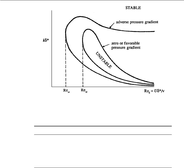
518 Instability
Figure 12.24 Sketch of marginal stability curves for a boundary layer with favorable and adverse pressure
gradients.
TABLE 12.1 Linear Stability Results of Common Viscous Parallel Flows
Flow U(y)/U
0
Re
cr
Remarks
Jet sech
2
( y/L) 4
Shear layer tanh ( y/L) 0 Always unstable
Blasius 520 Re based on δ
∗
Plane Poiseuille 1 −( y/L)
2
5780 L = half-width
Pipe flow 1 − (r/R)
2
∞ Always stable
Plane Couette y/L ∞ Always stable
layer calculation (Figure 12.23). Note also that the critical Reynolds number is lower
for flows with adverse pressure gradients.
Table 12.1 summarizes the results of the linear stability analyses of some common
parallel viscous flows.
The first two flows in the table have points of inflection in the velocity profile
and are inviscidly unstable; the viscous solution shows either a zero or a small critical
Reynolds number. The remaining flows are stable in the inviscid limit. Of these, the
Blasius boundary layer and the plane Poiseuille flow are unstable in the presence of
viscosity, but have high critical Reynolds numbers.
In Section 10.17 we discussed the decay of a laminar shear layer. Mass conser-
vation requires that a transverse velocity be generated so the flow cannot be parallel.
Although the idealized tanh profile for a shear layer, assuming straight and parallel
streamlines is immediately unstable, recent work by Bhattacharya et al. (2006), which
allowed for the basic flow to be two-dimensional, has yielded a finite critical Reynolds
number, modifying somewhat Table 12.1 (above).
10. Some Results of Parallel Viscous Flows 519
How can Viscosity Destabilize a Flow?
Let us examine how viscous effects can be destabilizing. For this we derive an integral
form of the kinetic energy equation in a viscous flow. The Navier–Stokes equation
for the disturbed flow is
∂
∂t
(U
i
+ u
i
) + (U
j
+ u
j
)
∂
∂x
j
(U
i
+ u
i
)
=−
1
ρ
∂
∂x
i
(P + p) + ν
∂
2
∂x
j
∂x
j
(U
i
+ u
i
).
Subtracting the equation of motion for the basic state, we obtain
∂u
i
∂t
+ u
j
∂u
i
∂x
j
+ U
j
∂u
i
∂x
j
+ u
j
∂U
i
∂x
j
=−
1
ρ
∂p
∂x
i
+ ν
∂
2
u
i
∂x
2
j
,
which is the equation of motion of the disturbance. The integrated mechanical energy
equation for the disturbance motion is obtained by multiplying this equation by u
i
and integrating over the region of flow. The control volume is chosen to coincide with
the walls where no-slip conditions are satisfied, and the length of the control volume
in the direction of periodicity is chosen to be an integral number of wavelengths
(Figure 12.25). The various terms of the energy equation then simplify as follows:
u
i
∂u
i
∂t
dV =
d
dt
u
2
i
2
dV,
u
i
u
j
∂u
i
∂x
j
dV =
1
2
∂
∂x
j
(u
2
i
u
j
)dV =
1
2
u
2
i
u
j
dA
j
= 0,
u
i
U
j
∂u
i
∂x
j
dV =
1
2
∂
∂x
j
(u
2
i
U
j
)dV =
1
2
u
2
i
U
j
dA
j
= 0,
u
i
∂p
∂x
i
dV =
∂
∂x
i
(pu
i
)dV =
pu
i
dA
i
= 0,
u
i
∂
2
u
i
∂x
2
j
dV =
∂
∂x
j
u
i
∂u
i
∂x
j
dV −
∂u
i
∂x
j
∂u
i
∂x
j
dV
=−
∂u
i
∂x
j
∂u
i
∂x
j
dV.
Here, dA is an element of surface area of the control volume, and dV is an
element of volume. In these the continuity equation ∂u
i
/∂x
i
= 0, Gauss’ theorem,
and the no-slip and periodic boundary conditions have been used to show that the
divergence terms drop out in an integrated energy balance. We finally obtain
d
dt
1
2
u
2
i
dV =−
u
i
u
j
∂U
i
∂x
j
dV − φ,
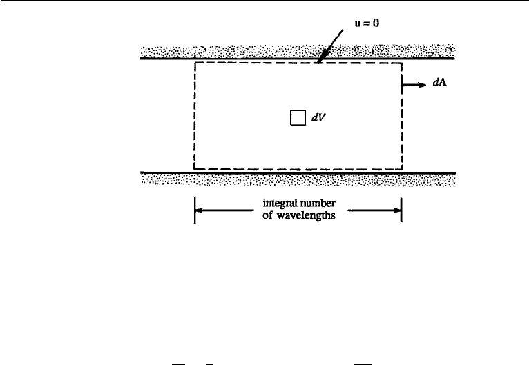
520 Instability
Figure 12.25 A control volume with zero net flux across boundaries.
where φ = ν
(∂u
i
/∂x
i
)
2
dV is the viscous dissipation. For two-dimensional dis-
turbances in a shear flow defined by U =[U(y),0, 0], the energy equation
becomes
d
dt
1
2
(u
2
+ v
2
)dV =−
uv
∂U
∂y
dV − φ. (12.83)
This equation has a simple interpretation. The first term is the rate of change of kinetic
energy of the disturbance, and the second term is the rate of production of disturbance
energy by the interaction of the “Reynolds stress” uv and the mean shear ∂U/∂y. The
concept of Reynolds stress will be explained in the following chapter. The point to
note here is that the value of the product uv averaged over a period is zero if the
velocity components u and v are out of phase of 90
◦
; for example, the mean value of
uv is zero if u = sin t and v = cos t.
In inviscid parallel flows without a point of inflection in the velocity profile, the
u and v components are such that the disturbance field cannot extract energy from
the basic shear flow, thus resulting in stability. The presence of viscosity, however,
changes the phase relationship between u and v, which causes Reynolds stresses such
that the mean value of −uv(∂U/∂y) over the flow field is positive and larger than the
viscous dissipation. This is how viscous effects can cause instability.
11. Experimental Verification of Boundary Layer Instability
In this section we shall present the results of stability calculations of the Blasius
boundary layer profile and compare them with experiments. Because of the nearly
parallel nature of the Blasius flow, most stability calculations are based on an analysis
of the Orr–Sommerfeld equation, which assumes a parallel flow. The first calculations
were performed by Tollmien in 1929 and Schlichting in 1933. Instead of assuming

11. Experimental Verification of Boundary Layer Instability 521
exactly the Blasius profile (which can be specified only numerically), they used the
profile
U
U
∞
=
1.7( y/δ) 0 y/δ 0.1724,
1 − 1.03 [1 − ( y/δ)
2
] 0.1724 y/δ 1,
1 y/δ 1,
which, like the Blasius profile, has a zero curvature at the wall. The calculations
of Tollmien and Schlichting showed that unstable waves appear when the Reynolds
number is high enough; the unstable waves in a viscous boundary layer are called
Tollmien–Schlichting waves. Until 1947 these waves remained undetected, and the
experimentalists of the period believed that the transition in a real boundary layer was
probably a finite amplitude effect. The speculation was that large disturbances cause
locally adverse pressure gradients, which resulted in a local separation and consequent
transition. The theoretical view, in contrast, was that small disturbances of the right
frequency or wavelength can amplify if the Reynolds number is large enough.
Verification of the theory was finally provided by some clever experiments con-
ducted by Schubauer and Skramstad in 1947. The experiments were conducted in
a “low turbulence” wind tunnel, specially designed such that the intensity of fluc-
tuations of the free stream was small. The experimental technique used was novel.
Instead of depending on natural disturbances, they introduced periodic disturbances
of known frequency by means of a vibrating metallic ribbon stretched across the flow
close to the wall. The ribbon was vibrated by passing an alternating current through it
in the field of a magnet. The subsequent development of the disturbance was followed
downstream by hot wire anemometers. Such techniques have now become standard.
The experimental data are shown in Figure 12.26, which also shows the
calculations of Schlichting and the more accurate calculations of Shen. Instead of
the wavenumber, the ordinate represents the frequency of the wave, which is easier
to measure. It is apparent that the agreement between Shen’s calculations and the
experimental data is very good.
The detection of the Tollmien–Schlichting waves is regarded as a major accom-
plishment of the linear stability theory. The ideal conditions for their existence require
two dimensionality and consequently a negligible intensity of fluctuations of the free
stream. These waves have been found to be very sensitive to small deviations from
the ideal conditions. That is why they can be observed only under very carefully
controlled experimental conditions and require artificial excitation. People who care
about historical fairness have suggested that the waves should only be referred to as
TS waves, to honor Tollmien, Schlichting, Schubauer, and Skramstad. The TS waves
have also been observed in natural flow (Bayly et al., 1988).
Nayfeh and Saric (1975) treated Falkner-Skan flows in a study of nonparallel
stability and found that generally there is a decrease in the critical Reynolds number.
The decrease is least for favorable pressure gradients, about 10% for zero pressure gra-
dient, and grows rapidly as the pressure gradient becomes more adverse. Grabowski
(1980) applied linear stability theory to the boundary layer near a stagnation point
on a body of revolution. His stability predictions were found to be close to those of
parallel flow stability theory obtained from solutions of the Orr–Sommerfeld equation.