Cohen I.M., Kundu P.K. Fluid Mechanics

Подождите немного. Документ загружается.

572 Turbulence

where τ

is the shear stress at the wall. To express equation (13.47) in terms of

dimensionless variables, note that only ρ and τ

involve the dimension of mass, so

that these two variables must always occur together in any nondimensional group.

The important ratio

∗

≡



(13.48)

has the dimension of velocity and is called the friction velocity. Equation (13.47) can

then be written as

U = U(u

∗

,ν,y). (13.49)

This relates four variables involving only the two dimensions of length and time.

According to the pi theorem (Chapter 8, Section 4) there must be only 4 − 2 = 2

nondimensional groups U/u

∗

and yu

∗

/ν, which should be related by some universal

functional form

∗

= f



∗



= f(y

) (law of the wall), (13.50)

where y

≡ yu

∗

/ν is the distance nondimensionalized by the viscous scale ν/u

∗

Equation (13.50) is called the law of the wall, and states that U/u

∗

must be a universal

function of yu

∗

/ν near a smooth wall.

The inner part of the wall layer, right next to the wall, is dominated by viscous

effects (Figure 13.18) and is called the viscous sublayer. It used to be called the

“laminar sublayer,” until experiments revealed the presence of considerable ﬂuctu-

ations within the layer. In spite of the ﬂuctuations, the Reynolds stresses are still

small here because of the dominance of viscous effects. Because of the thinness of

the viscous sublayer, the stress can be taken as uniform within the layer and equal

to the wall shear stress τ

. Therefore the velocity gradient in the viscous sublayer is

given by

= τ

which shows that the velocity distribution is linear. Integrating, and using the no-slip

boundary condition, we obtain

U =

yτ

In terms of nondimensional variables appropriate for a wall layer, this can be written as

∗

= y

(viscous sublayer). (13.51)

Experiments show that the linear distribution holds up to yu

∗

/ν ∼ 5, which may be

taken to be the limit of the viscous sublayer.

11. Wall-Bounded Shear Flow 573

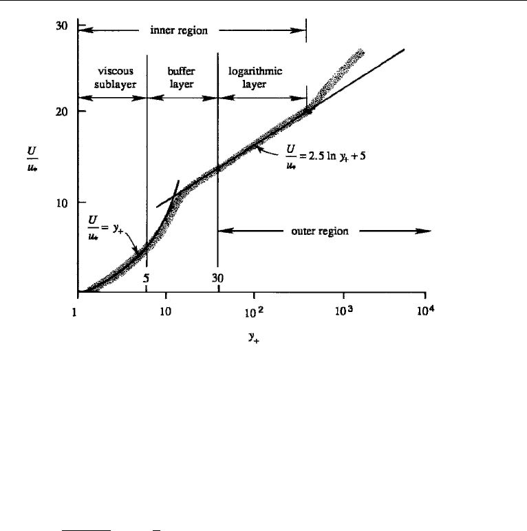
Figure 13.18 Law of the wall. A typical data cloud is shaded.

Outer Layer: Velocity Defect Law

We now explore the form of the velocity distribution in the outer part of a turbulent

layer. The gross characteristics of the turbulence in the outer region are inviscid and

resemble those of a wall-free turbulent ﬂow. The existence of Reynolds stresses in the

outer region results in a drag on the ﬂow and generates a velocity defect (U

∞

− U),

which is expected to be proportional to the wall friction characterized by u

∗

. It follows

that the velocity distribution in the outer region must have the form

U − U

∞

∗

= F





= F(ξ) (velocity defect law), (13.52)

where ξ ≡ y/δ. This is called the velocity defect law.

Overlap Layer: Logarithmic Law

The velocity proﬁles in the inner and outer parts of the boundary layer are governed

by different laws (13.50) and (13.52), in which the independent variable y is scaled

differently. Distances in the outer part are scaled by δ, whereas those in the inner part

are measured by the much smaller viscous scale ν/u

∗

. In other words, the small dis-

tances in the inner layer are magniﬁed by expressing them as yu

∗

/ν. This is the typical

behavior in singular perturbation problems (see Chapter 10, Sections 14 and 16). In

these problems the inner and outer solutions are matched together in a region of over-

lap by taking the limits y

→∞and ξ → 0 simultaneously. Instead of matching

velocity, in this case it is more convenient to match their gradients. (The derivation

574 Turbulence

given here closely follows Tennekes and Lumley (1972).) From equations (13.50)

and (13.52), the velocity gradients in the inner and outer regions are given by

∗

, (13.53)

∗

dξ

. (13.54)

Equating (13.53) and (13.54) and multiplying by y/u

∗

, we obtain

dξ

= y

, (13.55)

valid for large y

and small ξ . As the left-hand side can only be a function of ξ and

the right-hand side can only be a function of y

, both sides must be equal to the same

universal constant, say 1/k, where k is called the von Karman constant. Experiments

show that k  0.41. Integration of equation (13.55) gives

f(y

) =

ln y

+ A,

F(ξ) =

ln ξ +B.

(13.56)

Experiments show that A = 5.0 and B =−1.0 for a smooth ﬂat plate, for which

equations (13.56) become

∗

+ 5.0,

U − U

∞

∗

− 1.0.

(13.57)

(13.58)

These are the velocity distributions in the overlap layer, also called the inertial sub-

layer or simply the logarithmic layer. As the derivation shows, these laws are only

valid for large y

and small y/δ.

The foregoing method of justifying the logarithmic velocity distribution near a

wall was ﬁrst given by Clark B. Millikan in 1938, before the formal theory of singular

perturbation problems was fully developed. The logarithmic law, however, was known

from experiments conducted by the German researchers, and several derivations based

on semiempirical theories were proposed by Prandtl and von Karman. One such

derivation by the so-called mixing length theory is presented in the following section.

The logarithmic velocity distribution near a surface can be derived solely on

dimensional grounds. In this layer the velocity gradient dU/dy can only depend on

the local distance y and on the only relevant velocity scale near the surface, namely u

∗

(The layer is far enough from the wall so that the direct effect of ν is not relevant

and far enough from the outer part of the turbulent layer so that the effect of δ is not

11. Wall-Bounded Shear Flow 575

relevant.) A dimensional analysis gives

∗

where the von Karman constant k is introduced for consistency with the preceding

formulas. Integration gives

U =

∗

ln y + const. (13.59)

It is therefore apparent that dimensional considerations alone lead to the logarithmic

velocity distribution near a wall. In fact, the constant of integration can be adjusted

to reduce equation (13.59) to equation (13.57) or (13.58). For example, matching the

proﬁle to the edge of the viscous sublayer at y = 10.7ν/u

∗

reduces equation (13.59)

to equation (13.57) (Exercise 8). The logarithmic velocity distribution also applies to

rough walls, as discussed later in the section.

The experimental data on the velocity distribution near a wall is sketched in

Figure 13.18. It is a semilogarithmic plot in terms of the inner variables. It shows that

the linear velocity distribution (13.51) is valid for y

< 5, so that we can take the

viscous sublayer thickness to be



5ν

∗

(viscous sublayer thickness).

The logarithmic velocity distribution (13.57) is seen to be valid for 30 <y

< 300.

The upper limit on y

, however, depends on the Reynolds number and becomes

larger as Re increases. There is therefore a large logarithmic overlap region in ﬂows

at large Reynolds numbers. The close analogy between the overlap region in physical

space and inertial subrange in spectral space is evident. In both regions, there is little

production or dissipation; there is simply an “inertial” transfer across the region by

inviscid nonlinear processes. It is for this reason that the logarithmic layer is called

the inertial sublayer.

As equation (13.58) suggests, a logarithmic velocity distribution in the overlap

region can also be plotted in terms of the outer variables of (U − U

∞

)/u

∗

vs y/δ.

Such plots show that the logarithmic distribution is valid for y/δ < 0.2. The loga-

rithmic law, therefore, holds accurately in a rather small percentage (∼20%) of the

total boundary layer thickness. The general defect law (13.52), where F(ξ) is not

necessarily logarithmic, holds almost everywhere except in the inner part of the wall

layer.

The region 5 <y

< 30, where the velocity distribution is neither linear nor

logarithmic, is called the buffer layer. Neither the viscous stress nor the Reynolds

stress is negligible here. This layer is dynamically very important, as the turbulence

production −

uv(dU/dy) reaches a maximum here due to the large velocity gradients.

Wosnik et al. (2000) very carefully reexamined turbulent pipe and channel ﬂows

and compared their results with superpipe data and scalings developed by Zagarola

and Smits (1998), and others. Very brieﬂy, Figure 13.18 is split into more regions

576 Turbulence

in that a “mesolayer” is required between the buffer layer and the inertial sublayer.

Proper description of the velocity in this mesolayer requires an offset parameter in the

logarithm of equations (13.56). This is obtained by generalizing equation (13.55) to

(ξ +¯a)

d(ξ +¯a)

= (y

+ a

)

d(y

+ a

)

where ¯a = a/δ, a

= au

∗

/ν.

Equations (13.56) become

f(y

) = k

−1

ln(y

+ a

) + A,

F(ξ) = k

−1

ln(ξ +¯a) +B.

The value for a

suggested by Wosnik et al. that best ﬁts the superpipe data is

=−8.

A more rational asymptotic treatment was given by Buschmann and Gad-el-Hak

(2003a) in terms of an expansion for large Karman number δ



/2)·(δ/θ )Re

in the case of a zero pressure gradient turbulent boundary layer. Here C

is the

skin friction coefﬁcient deﬁned in (10.38) and θ is the momentum thickness deﬁned

in (10.17). Re

is the Reynolds number based on the local momentum thickness of

the boundary layer. The second author had previously found δ

= 1.168(Re

)

.875

empirically over a wide range of Re. U/u

∗

is expanded in both the inner layer (y

)

and the outer layer (η = y/δ) in negative powers of δ

. To lowest order we recover the

simple log velocity proﬁle [(13.59)]. Higher-order terms include powers of the inner

and outer variables. After matching in an overlap region, the remaining coefﬁcients

are ultimately determined by comparison with experiments. Comparing with alter-

native forms for the turbulent velocity proﬁles, Buschmann and Gad-el-Hak (2003b)

conclude that the generalized log law gives a better ﬁt over an extended range of y

than any alternative velocity proﬁle. Also, as Re

increases, the higher-order terms in

the Karman number expansion become asymptotically small.

The outer region of turbulent boundary layers (y

> 100) is the subject of a

similarity analysis by Castillo and George (2001). They found that 90% of a turbu-

lent ﬂow under all pressure gradients is characterized by a single pressure gradient

parameter,

 =

ρU

∞

dδ/dx

∞

A requirement for “equilibrium” turbulent boundary layer ﬂows, to which their anal-

ysis is restricted, is that  = const., and this leads to similarity. Examination of

data from many sources led them to conclude that “...there appear to be almost

no ﬂows that are not in equilibrium ....” Their most remarkable result is that only

three values of  correlate the data for all pressure gradients:  = 0.22 (adverse

pressure gradients);  =−1.92 (favorable pressure gradients); and  = 0 (zero

pressure gradient). A direct consequence of  = const. is that δ(x) ∼ U

−1/

∞

. Data

was well correlated by this result for both favorable and adverse pressure gradients.

Walker and Castillo (2002) then correlated velocity defect proﬁles for favorable, zero,

11. Wall-Bounded Shear Flow 577

and adverse pressure gradients by plotting

[

∞

− U)/U

∞

]

(δ

∗

/δ

) vs. y/δ

. (See

Section 10.3 for the deﬁnitions of δ

and δ

∗

). Remarkably, only three distinct tur-

bulent velocity proﬁles resulted. This correlation of data with only three values of

 was contested by Maciel, Rossignol, and Lemay (2006) in their examination of

data bases for adverse pressure gradient turbulent boundary layers. They found that

scalings developed by Zagarola and Smits (1998) worked best but that  varied by a

factor of 2 (from 0.16 to 0.33), while in each of the ﬂows  was held constant and

the ﬂow was observed to be self-similar. The value of  = 0.22 held for only two

of the nine adverse pressure gradient data sets listed by Maciel et al. Moreover, the

velocity defect proﬁles for adverse pressure gradient ﬂows did not collapse onto a

single limiting proﬁle, as asserted by Walker and Castillo.

Very close to separation, the boundary layer assumptions that ∂/∂x  ∂/∂y and

v  u break down and new scalings become necessary as discussed in Indinger,

Buschmann, and Gad-el-Hak (2006).

A review paper by W. K. George (2006) puts much of the analysis and discussion

into a wide-view perspective. Three scalings for the outer 90% of the zero pressure

gradient turbulent velocity deﬁcit proﬁles are written, the ﬁrst a generalization of

Eq. (13.52) to include behavior with δu

∗

/ν. The second is of the same form but the

normalization is by U

∞

instead of u

∗

. The third scaling is of the form of the second

with the functional behavior prefaced by δ

∗

/δ, where the displacement thickness

∗

is deﬁned in Eq. (10.16). The ﬁrst scaling gives the logarithmic behavior in the

overlap between the inner and outer regions of the turbulent boundary layer whereas

the second gives a power law.

Professor George pointed out that although the momentum integral equation for

constant pressure turbulent boundary layers [Eq. (10.44)] holds, dθ/dx = (u

∗

∞

)

and the main contribution to θ [momentum thickness, Eq. (10.17)] comes from near

wall regions, almost the entire value of dθ/dx comes from distances far from the

wall.

The third scaling is due to Zagarola and Smits (1998) and can reduce to either

of the ﬁrst two depending on the Re →∞asymptotic behavior. If δ

∗

/δ → u

∗

∞

then the ﬁrst scaling leading to a logarithmic overlap is obtained. If, on the other

hand, δ

∗

/δ → const., then the second scaling leading to a power law is found. Here

the limit Re →∞must be taken as x →∞downstream with ﬁxed upstream and

external conditions. It is also shown here that the logarithmic overlap is the lowest

order in an expansion of the power law. The two results are very close largely because

du/dy ∼ 1/y

yields a logarithm (upon integration) but du/dy ∼ 1/y

where γ is

anything other than = 1 but may be very close to 1, yields a power upon integration.

Since the latter is more general and results from a difference in turbulence scales in

the two regions involved in the overlap, it is likely to be correct, but more detailed

and careful data is required to distinguish the two forms.

It is easier to discuss the details of the balance among regions of turbulence for

a planar fully developed pressure driven turbulent shear ﬂow. Consider a ﬂow in the

x-direction between two parallel plates at y = 0 and y = 2δ that is no longer evolving

in the x-direction. The convective acceleration terms are then identically zero and the

x-momentum equation reduces to −∂P/∂x +d/dy(µ∂U/∂y −ρ

uv) = 0 . Since the

578 Turbulence

pressure gradient is constant in x, it must be balanced by the shear stress on the two

walls over any distance L, which yields the equality τ

=−δ ·∂P/∂x. Then with the

dimensionless variables, U/u

∗

= u

, yu

∗

/ν = y

, δu

∗

/v = δ

,(uv)/u

∗

= (uv)

the x-momentum equation becomes δ

−1

+ d

/dy

− d/dy(uv)

= 0, represent-

ing a balance among the pressure gradient, viscous stress gradient, and Reynolds

stress gradient. This is the starting point of the analysis by Fife, Wei, Klewicki, and

McMurtry (2005). The authors ﬁnd distinct scalings representing different balances

of terms. These are described by the following in order of increasing distance from

the wall. For y

< 3, there is the sublayer where the viscous stress gradient balances

the mean pressure gradient, and the Reynolds stress gradient is small by comparison.

As we go outwards from the wall, the viscous stress gradient balances the Reynolds

stress gradient. For large enough Re this layer extends into the logarithmic region of

the earlier models. Near the location of maximum Reynolds stress, since the Reynolds

stress gradient is small, the viscous stress gradient and pressure gradient are again in

balance. This is true despite the Reynolds stress being much larger than the viscous

stress. This region is called the viscous/pressure gradient mesolayer. Still further from

the wall the Reynolds stress gradient and pressure gradient are in balance.

Wei, Fife, and Klewicki (2007) codiﬁed this analysis for any combination of

Couette and Poiseuille ﬂows. We will concentrate on the latter. Explicitly, the inner

normalized equations are written in terms of u

and y

. The innermost viscous layer

is then a simple generalization of Eq. (13.51) to include the pressure gradient. The

balance of the inner normalized equations is between the viscous and Reynolds stress

gradients. The outer normalization retains u

but uses ξ = y/δ as the outer length

scale. In the outermost region, the Reynolds stress and pressure gradients balance

giving: 1 − d/dξ(

uv)

= O(δ

−1

) → 0. Between these, in the neighborhood of

maximum Reynolds stress, there is a mesolayer in which all terms are in balance.

This is scaled by:

y = (y

− y

)δ

−1/2



uv) = δ

1/2



(

uv)

− (uv)



= u

− u

− (du

/dy

)

·(y

− y

Here, all ˆvariables are ﬁnite in the limit δ

≡ Re

∗

→∞. Although the location y

and the value of (uv)

are not known a priori, good approximations are obtained if

−1/2

= 1 and (uv)

= 1.

Fife et al. (2005) and Wei et al. (2007) introduced the notion of scaling patches

such that a patch is “...deﬁned to be a region in the ﬂow ﬁeld speciﬁed by an interval

of distance from the wall, together with a scaling or non-dimensionalization of the

variables which is natural for that region.” Here “natural” means that in appropriately

normalized variables, the data within that region are independent of Reynolds number

in the turbulent limit, Re →∞. The authors assert that knowledge of the local

scaling properties of the mean momentum and Reynolds stress proﬁles is essential to

understanding wall bounded turbulent ﬂows. The scaling to render all three terms in

the mean momentum balance of the same order (in Re or δ

) in the neighborhood

of the Reynolds stress maximum is indeterminate, leaving one free parameter. All

coefﬁcients are = 1 in the Re →∞limit in this patch centered about the Reynolds

11. Wall-Bounded Shear Flow 579

stress maximum. A very special choice of this free parameter leads to a logarithm

for u

; any other choice gives power law growth. A different scaling patch may be

found in the neighborhood of the channel centerline, again with one free parameter.

A very special choice of the free parameter results in the classical defect law for the

outermost layer.

Rough Surface

In deriving the logarithmic law (13.57), we assumed that the ﬂow in the inner layer

is determined by viscosity. This is true only in hydrodynamically smooth surfaces,

for which the average height of the surface roughness elements is smaller than the

thickness of the viscous sublayer. For a hydrodynamically rough surface, on the other

hand, the roughness elements protrude out of the viscous sublayer. An example is

the ﬂow near the surface of the earth, where the trees and buildings act as rough-

ness elements. This causes a wake behind each roughness element, and the stress is

transmitted to the wall by the “pressure drag” on the roughness elements. Viscosity

becomes irrelevant for determining either the velocity distribution or the overall drag

on the surface. This is why the drag coefﬁcients for a rough pipe and a rough ﬂat

surface become independent of the Reynolds number as Re →∞.

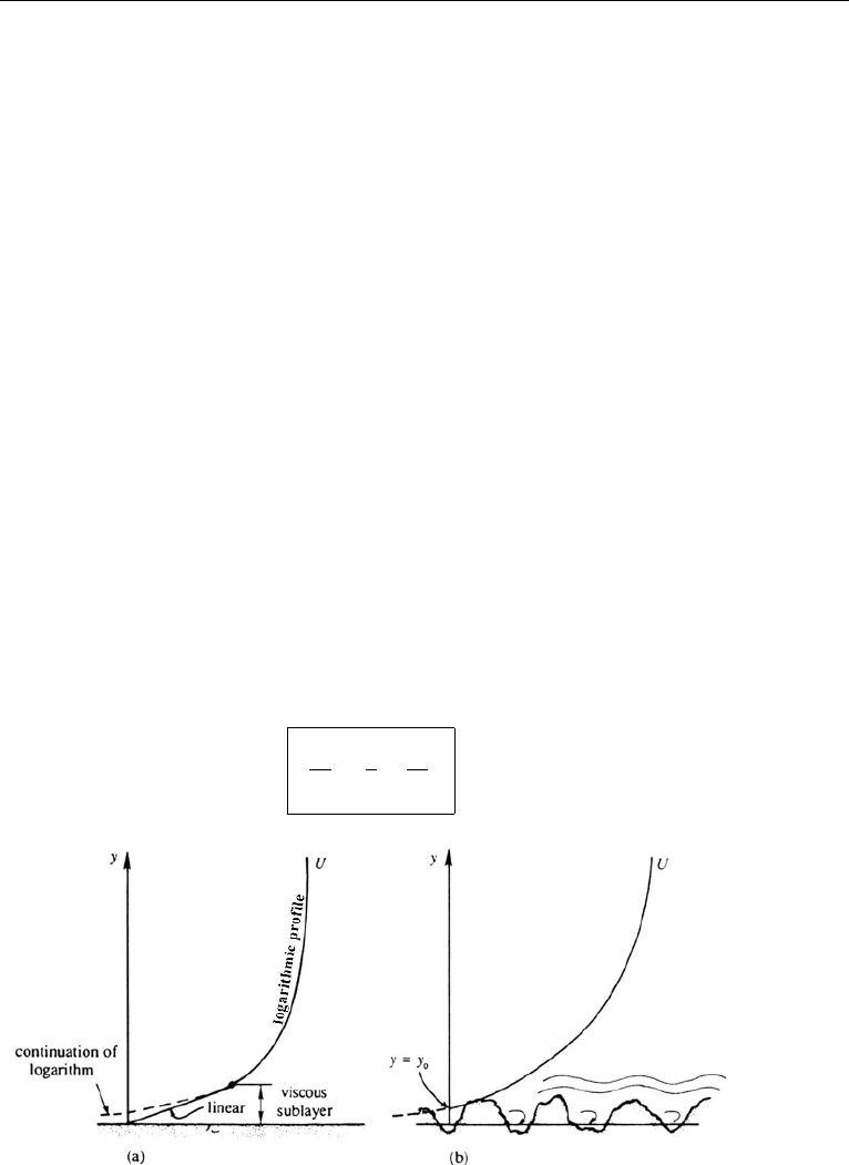
The velocity distribution near a rough surface is again logarithmic, although it

cannot be represented by equation (13.57). To ﬁnd its form, we start with the general

logarithmic law (13.59). The constant of integration can be determined by noting that

the mean velocity U is expected to be negligible somewhere within the roughness

elements (Figure 13.19b). We can therefore assume that (13.59) applies for y>y

where y

is a measure of the roughness heights and is deﬁned as the value of y at

which the logarithmic distribution gives U = 0. Equation (13.59) then gives

∗

. (13.60)

Figure 13.19 Logarithmic velocity distributions near smooth and rough surfaces: (a) smooth wall; and

(b) rough wall.

580 Turbulence

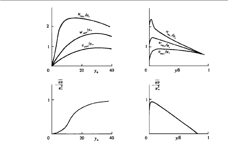
Figure 13.20 Sketch of observed variation of turbulent intensity and Reynolds stress across a channel

of half-width δ. The left panels are plots as functions of the inner variable y

, while the right panels are

plots as functions of the outer variable y/δ.

Variation of Turbulent Intensity

The experimental data of turbulent intensity and Reynolds stress in a channel ﬂow are

given in Townsend (1976). Figure 13.20 shows a schematic representation of these

data, plotted both in terms of the outer and the inner variables. It is seen that the

turbulent velocity ﬂuctuations are of order u

∗

. The longitudinal ﬂuctuations are the

largest because the shear production initially feeds the energy into the u-component;

the energy is subsequently distributed into the lateral components v and w. (Inciden-

tally, in a convectively generated turbulence the turbulent energy is initially fed to the

vertical component.) The turbulent intensity initially rises as the wall is approached,

but goes to zero right at the wall in a very thin wall layer. As expected from phys-

ical considerations, the normal component v

rms

starts to feel the wall effect earlier.

Figure 13.20 also shows that the distribution of each variable very close to the wall

becomes clear only when the distances are magniﬁed by the viscous scaling ν/u

∗

The Reynolds stress proﬁle in terms of the inner variable shows that the stresses are

negligible within the viscous sublayer (y

< 5), beyond which the Reynolds stress

is nearly constant throughout the wall layer. This is why the logarithmic layer is also

called the constant stress layer.

12. Eddy Viscosity and Mixing Length

The equations for mean motion in a turbulent ﬂow, given by equation (13.24), cannot

be solved for U

(x) unless we have an expression relating the Reynolds stresses

12. Eddy Viscosity and Mixing Length 581

in terms of the mean velocity ﬁeld. Prandtl and von Karman developed certain

semiempirical theories that attempted to provide this relationship.

These theories are based on an analogy between the momentum exchanges both

in turbulent and in laminar ﬂows. Consider ﬁrst a unidirectional laminar ﬂow U(y),

in which the shear stress is

lam

= ν

, (13.61)

where ν is a property of the ﬂuid.According to the kinetic theory of gases, the diffusive

properties of a gas are due to the molecular motions, which tend to mix momentum

and heat throughout the ﬂow. It can be shown that the viscosity of a gas is of order

ν ∼ aλ, (13.62)

where a is the rms speed of molecular motion, and λ is the mean free path deﬁned as

the average distance traveled by a molecule between collisions. The proportionality

constant in equation (13.62) is of order 1.

One is tempted to speculate that the diffusive behavior of a turbulent ﬂow may

be qualitatively similar to that of a laminar ﬂow and may simply be represented by a

much larger diffusivity. By analogy with (13.61), Boussinesq proposed to represent

the turbulent stress as

−

uv = ν

, (13.63)

where ν

is the eddy viscosity. Note that, whereas ν is a known property of the ﬂuid, ν

in (13.63) depends on the conditions of the ﬂow. We can always divide the turbulent

stress by the mean velocity gradient and call it ν

, but this is not progress unless

we can formulate a rational method for ﬁnding the eddy viscosity from other known

parameters of a turbulent ﬂow.

The eddy viscosity relation (13.63) implies that the local gradient determines

the ﬂux. However, this cannot be valid if the eddies happen to be larger than the

scale of curvature of the proﬁle. Following Panofsky and Dutton (1984), consider the

atmospheric concentration proﬁle of carbon monoxide (CO) shown in Figure 13.21.

An eddy viscosity relation would have the form

−

wc = κ

, (13.64)

where C is the mean concentration (kilograms of CO per kilogram of air), c is its

ﬂuctuation, and κ

is the eddy diffusivity. A positive κ

requires that the ﬂux of CO at

P be downward. However, if the thermal convection is strong enough, the large eddies

so generated can carry large amounts of CO from the ground to point P, and result in

an upward ﬂux there. The direction of ﬂux at P in this case is not determined by the

local gradient at P, but by the concentration difference between the surface and point

P. In this case, the eddy diffusivity found from equation (13.64) would be negative

and, therefore, not very meaningful.