Cohen I.M., Kundu P.K. Fluid Mechanics

Подождите немного. Документ загружается.

562 Turbulence

(which may be taken equal to the rms ﬂuctuating speed). Then the time scale of large

eddies is of order l/u



. Observations show that the large eddies lose much of their

energy during the time they turn over one or two times, so that the rate of energy

transferred from large eddies is proportional to u

2

times their frequency u



/l. The

dissipation rate must then be of order

ε ∼

3

(13.38)

signifying that the viscous dissipation is determined by the inviscid large-scale

dynamics of the turbulent ﬁeld.

Kolmogorov suggested in 1941 that the size of the dissipating eddies depends

on those parameters that are relevant to the smallest eddies. These parameters are the

rate ε at which energy has to be dissipated by the eddies and the diffusivity ν that

does the smearing out of the velocity gradients. As the unit of ε is m

, dimensional

reasoning shows that the length scale formed from ε and ν is

η =





1/4

(13.39)

which is called the Kolmogorov microscale. A decrease of ν merely decreases the scale

at which viscous dissipation takes place, and not the rate of dissipation ε. Estimates

show that η is of the order of millimeters in the ocean and the atmosphere. In laboratory

ﬂows the Kolmogorov microscale is much smaller because of the larger rate of viscous

dissipation. Landahl and Mollo-Christensen (1986) give a nice illustration of this.

Suppose we are using a 100-W household mixer in 1 kg of water. As all the power is

used to generate the turbulence, the rate of dissipation is ε = 100 W/kg = 100 m

Using ν = 10

−6

/s for water, we obtain η = 10

−2

mm.

9. Spectrum of Turbulence in Inertial Subrange

In Section 4 we deﬁned the wavenumber spectrum S(K), representing turbulent

kinetic energy as a function of the wavenumber vector K. If the turbulence is isotropic,

then the spectrum becomes independent of the orientation of the wavenumber vector

and depends on its magnitude K only. In that case we can write



∞

S(K) dK.

In this section we shall derive the form of S(K) in a certain range of wavenumbers

in which the turbulence is nearly isotropic.

Somewhat vaguely, we shall associate a wavenumber K with an eddy of size K

−1

Small eddies are therefore represented by large wavenumbers. Suppose l is the scale

of the large eddies, which may be the width of the boundary layer. At the relatively

9. Spectrum of Turbulence in Inertial Subrange 563

small scales represented by wavenumbers K  l

−1

, there is no direct interaction

between the turbulence and the motion of the large, energy-containing eddies. This is

because the small scales have been generated by a long series of small steps, losing

information at each step. The spectrum in this range of large wavenumbers is nearly

isotropic, as only the large eddies are aware of the directions of mean gradients. The

spectrum here does not depend on how much energy is present at large scales (where

most of the energy is contained), or the scales at which most of the energy is present.

The spectrum in this range depends only on the parameters that determine the nature

of the small-scale ﬂow, so that we can write

S = S(K,ε, ν) K  l

−1

The range of wavenumbers K  l

−1

is usually called the equilibrium range. The

dissipating wavenumbers with K ∼ η

−1

, beyond which the spectrum falls off very

rapidly, form the high end of the equilibrium range (Figure 13.12). The lower end

of this range, for which l

−1

 K  η

−1

, is called the inertial subrange, as only

the transfer of energy by inertial forces (vortex stretching) takes place in this range.

Both production and dissipation are small in the inertial subrange. The production of

energy by large eddies causes a peak of S at a certain K  l

−1

, and the dissipation

of energy causes a sharp drop of S for K>η

−1

. The question is, how does S vary

with K between the two limits in the inertial subrange?

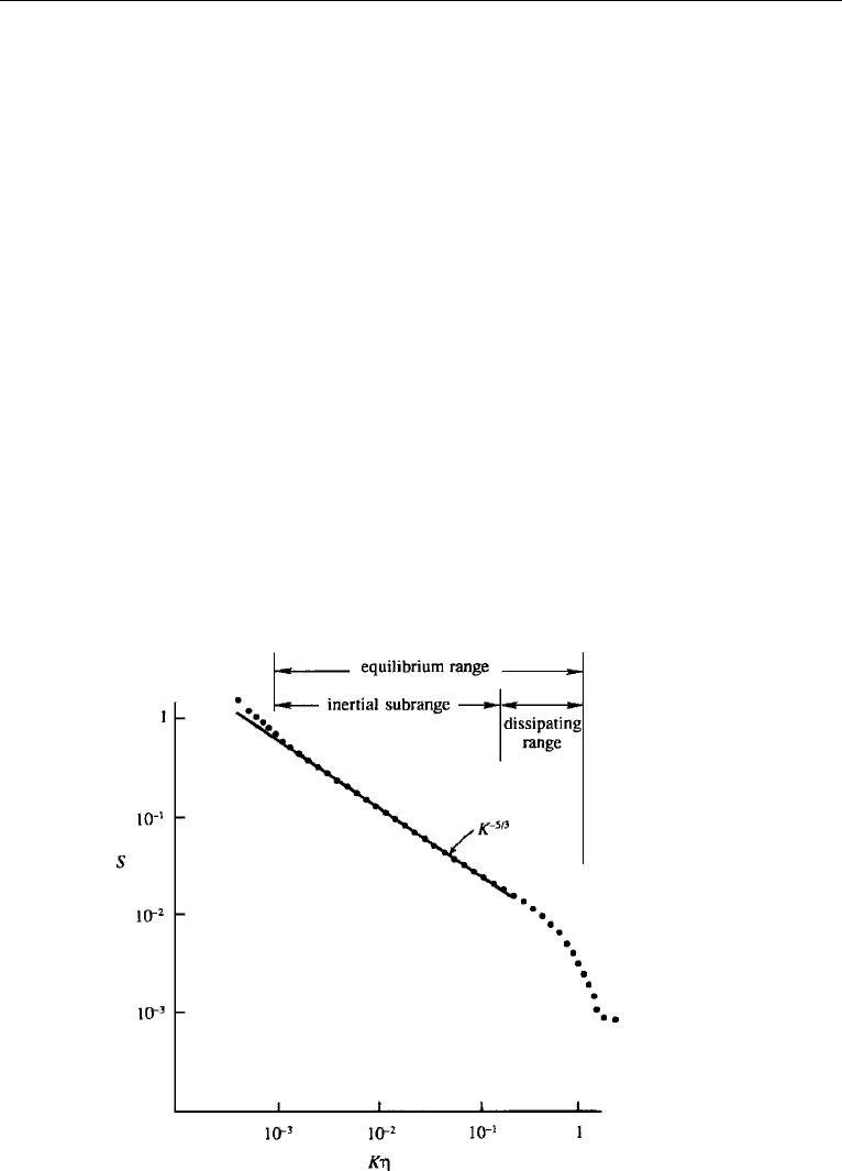
Figure 13.12 A typical wavenumber spectrum observed in the ocean, plotted on a log–log scale. The

unit of S is arbitrary, and the dots represent hypothetical data.

564 Turbulence

Kolmogorov argued that, in the inertial subrange part of the equilibrium range,

S is independent of ν also, so that

S = S(K,ε) l

−1

 K  η

−1

Although little dissipation takes place in the inertial subrange, the spectrum here does

depend on ε. This is because the energy that is dissipated must be transferred across

the inertial subrange, from low to high wavenumbers. As the unit of S is m

and

that of ε is m

, dimensional reasoning gives

S = Aε

2/3

−5/3

−1

 K  η

−1

, (13.40)

where A  1.5 has been found to be a universal constant, valid for all turbulent

ﬂows. Equation (13.40) is usually called Kolmogorov’s K

−5/3

law. If the Reynolds

number of the ﬂow is large, then the dissipating eddies are much smaller than the

energy-containing eddies, and the inertial subrange is quite broad.

Because very large Reynolds numbers are difﬁcult to generate in the laboratory,

the Kolmogorov spectral law was not veriﬁed for many years. In fact, doubts were

being raised about its theoretical validity. The ﬁrst conﬁrmation of the Kolmogorov

law came from the oceanic observations of Grant et al. (1962), who obtained a velocity

spectrum in a tidal ﬂow through a narrow passage between two islands near the west

coast of Canada. The velocity ﬂuctuations were measured by hanging a hot ﬁlm

anemometer from the bottom of a ship. Based on the depth of water and the average

ﬂow velocity, the Reynolds number was of order 10

. Such large Reynolds numbers

are typical of geophysical ﬂows, since the length scales are very large. The K

−5/3

law has since been veriﬁed in the ocean over a wide range of wavenumbers, a typical

behavior being sketched in Figure 13.12. Note that the spectrum drops sharply at

Kη ∼ 1, where viscosity begins to affect the spectral shape. The ﬁgure also shows

that the spectrum departs from the K

−5/3

law for small values of the wavenumber,

where the turbulence production by large eddies begins to affect the spectral shape.

Laboratory experiments are also in agreement with the Kolmogorov spectral law,

although in a narrower range of wavenumbers because the Reynolds number is not as

large as in geophysical ﬂows. The K

−5/3

law has become one of the most important

results of turbulence theory.

10. Wall-Free Shear Flow

Nearly parallel shear ﬂows are divided into two classes—wall-free shear ﬂows and

wall-bounded shear ﬂows. In this section we shall examine some aspects of turbulent

ﬂows that are free of solid boundaries. Common examples of such ﬂows are jets,

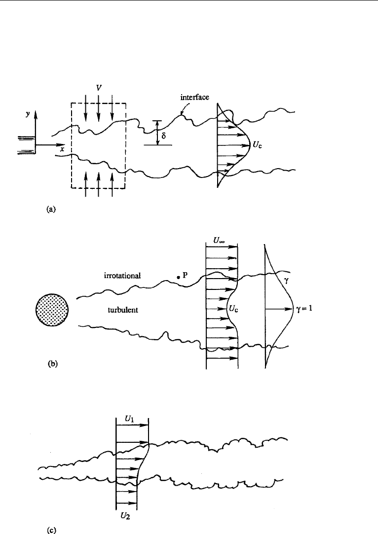
wakes, and shear layers (Figure 13.13). For simplicity we shall consider only plane

two-dimensional ﬂows. Axisymmetric ﬂows are discussed in Townsend (1976) and

Tennekes and Lumley (1972).

10. Wall-Free Shear Flow 565

Intermittency

Consider a turbulent ﬂow conﬁned to a limited region. To be speciﬁc we shall consider

the example of a wake (Figure 13.13b), but our discussion also applies to a jet, a shear

layer, or the outer part of a boundary layer on a wall. The ﬂuid outside the turbulent

Figure 13.13 Three types of wall-free turbulent ﬂows: (a) jet; (b) wake; and (c) shear layer.

566 Turbulence

region is either in irrotational motion (as in the case of a wake or a boundary layer), or

nearly static (as in the case of a jet). Observations show that the instantaneous interface

between the turbulent and nonturbulent ﬂuid is very sharp. In fact, the thickness of the

interface must equal the size of the smallest scales in the ﬂow, namely the Kolmogorov

microscale. The interface is highly contorted due to the presence of eddies of various

sizes. However, a photograph exposed for a long time does not show such an irregular

and sharp interface but rather a gradual and smooth transition region.

Measurements at a ﬁxed point in the outer part of the turbulent region (say at

point P in Figure 13.13b) show periods of high-frequency ﬂuctuations as the point P

moves into the turbulent ﬂow and quiet periods as the point moves out of the turbulent

region. Intermittency γ is deﬁned as the fraction of time the ﬂow at a point is turbulent.

The variation of γ across a wake is sketched in Figure 13.13b, showing that γ = 1

near the center where the ﬂow is always turbulent, and γ = 0 at the outer edge of

the ﬂow.

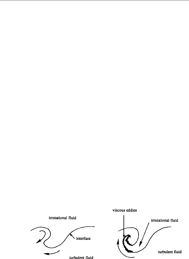
Entrainment

A ﬂow can slowly pull the surrounding irrotational ﬂuid inward by “frictional” effects;

the process is called entrainment. The source of this “friction” is viscous in laminar

ﬂow and inertial in turbulent ﬂow. The entrainment of a laminar jet was discussed in

Chapter 10, Section 12. The entrainment in a turbulent ﬂow is similar, but the rate is

much larger. After the irrotational ﬂuid is drawn inside a turbulent region, the new

ﬂuid must be made turbulent. This is initiated by small eddies (which are dominated

by viscosity) acting at the sharp interface between the turbulent and the nonturbulent

ﬂuid (Figure 13.14).

The foregoing discussion of intermittency and entrainment applies not only to

wall-free shear ﬂows but also to the outer edge of boundary layers.

Self-Preservation

Far downstream, experiments show that the mean ﬁeld in a wall-free shear ﬂow

becomes approximately self-similar at various downstream distances. As the mean

ﬁeld is affected by the Reynolds stress through the equations of motion, this means that

the various turbulent quantities (such as Reynolds stress) also must reach self-similar

Figure 13.14 Entrainment of a nonturbulent ﬂuid and its assimilation into turbulent ﬂuid by viscous

action at the interface.

10. Wall-Free Shear Flow 567

states. This is indeed found to be approximately true (Townsend, 1976). The ﬂow is

then in a state of “moving equilibrium,” in which both the mean and the turbulent

ﬁelds are determined solely by the local scales of length and velocity. This is called

self-preservation. In the self-similar state, the mean velocity at various downstream

distances is given by

= f





(jet),

∞

− U

∞

− U

= f





(wake),

U − U

− U

= f





(shear layer).

(13.41)

Here δ(x) is the width of ﬂow, U

(x) is the centerline velocity for the jet and the wake,

and U

are the velocities of the two streams in a shear layer (Figure 13.13).

Consequence of Self-Preservation in a Plane Jet

We shall now derive how the centerline velocity and width in a plane jet must vary if

we assume that the mean velocity proﬁles at various downstream distances are self

similar. This can be done by examining the equations of motion in differential form.

An alternate way is to examine an integral form of the equation of motion, derived in

Chapter 10, Section 12. It was shown there that the momentum ﬂux M = ρ



across the jet is independent of x, while the mass ﬂux ρ



Udyincreases downstream

due to entrainment. Exactly the same constraint applies to a turbulent jet. For the

sake of readers who ﬁnd cross references annoying, the integral constraint for a

two-dimensional jet is rederived here.

Consider a control volume shown by the dotted line in Figure 13.13a, in which the

horizontal surfaces of the control volume are assumed to be at a large distance from

the jet axis. At these large distances, there is a mean V ﬁeld toward the jet axis due to

entrainment, but no U ﬁeld. Therefore, the ﬂow of x-momentum through the horizon-

tal surfaces of the control volume is zero. The pressure is uniform throughout the ﬂow,

and the viscous forces are negligible. The net force on the surface of the control vol-

ume is therefore zero. The momentum principle for a control volume (see Chapter 4,

Section 8) states that the net x-directed force on the boundary equals the net rate of

outﬂow of x-momentum through the control surfaces. As the net force here is zero,

the inﬂux of x-momentum must equal the outﬂow of x-momentum. That is

M = ρ



∞

−∞

dy = independent of x, (13.42)

where M is the momentum ﬂux of the jet (=integral of mass ﬂux ρU dy times veloc-

ity U ). The momentum ﬂux is the basic externally controlled parameter for a jet and

is known from an evaluation of equation (13.42) at the oriﬁce opening. The mass ﬂux



Udyacross the jet must increase because of entrainment of the surrounding ﬂuid.

568 Turbulence

The assumption of self similarity can now be used to predict how δ and U

in a

jet should vary with x. Substitution of the self-similarity assumption (13.41) into the

integral constraint (13.42) gives

M = ρU



∞

−∞





The preceding integral is a constant because it is completely expressed in terms of

the nondimensional function f(y/δ).AsM is also a constant, we must have

δ = const. (13.43)

At this point we make another important assumption. We assume that the

Reynolds number is large, so that the gross characteristics of the ﬂow are independent

of the Reynolds number. This is called Reynolds number similarity. The assumption

is expected to be valid in a wall-free shear ﬂow, as viscosity does not directly affect

the motion; a decrease of ν, for example, merely decreases the scale of the dissipat-

ing eddies, as discussed in Section 8. (The principle is not valid near a smooth wall,

and as a consequence the drag coefﬁcient for a smooth ﬂat plate does not become

independent of the Reynolds number as Re →∞; see Figure 10.12.) For large Re,

then, U

is independent of viscosity and can only depend on x, ρ, and M:

= U

(x,ρ,M).

A dimensional analysis shows that

∝



ρx

( jet), (13.44)

so that equation (13.43) requires

δ ∝ x(jet). (13.45)

This should be compared with the δ ∝ x

2/3

behavior of a laminar jet, derived in

Chapter 10, Section 12. Experiments show that the width of a turbulent jet does grow

linearly, with a spreading angle of 4

◦

For two-dimensional wakes and shear layers, it can be shown (Townsend, 1976;

Tennekes and Lumley, 1972) that the assumption of self similarity requires

∞

− U

∝ x

−1/2

,δ∝

√

x (wake),

− U

= const., δ ∝ x (shear layer).

Turbulent Kinetic Energy Budget in a Jet

The turbulent kinetic energy equation derived in Section 7 will now be applied to

a two-dimensional jet. The energy budget calculation uses the experimentally mea-

sured distributions of turbulence intensity and Reynolds stress across the jet. There-

fore, we present the distributions of these variables ﬁrst. Measurements show that

10. Wall-Free Shear Flow 569

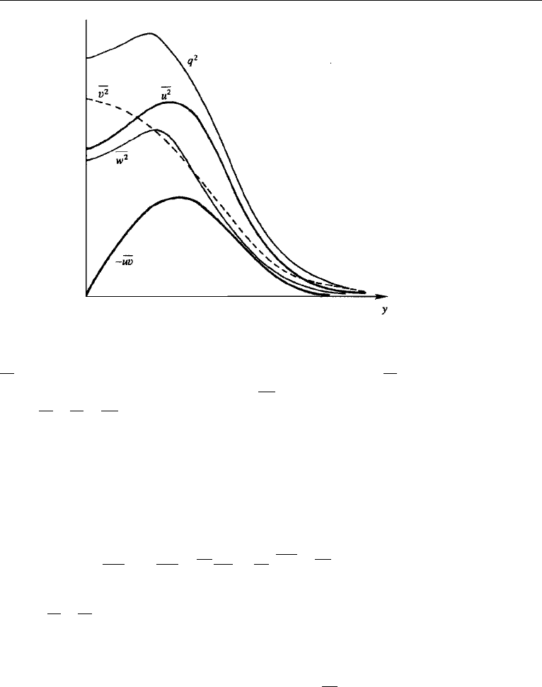
Figure 13.15 Sketch of observed variation of turbulent intensity and Reynolds stress across a jet.

the turbulent intensities and Reynolds stress are distributed as in Figure 13.15. Here

is the intensity of ﬂuctuation in the downstream direction x, v

is the inten-

sity along the cross-stream direction y, and

is the intensity in the z-direction;

≡ (u

+ v

+ w

)/2 is the turbulent kinetic energy per unit mass. The Reynolds

stress is zero at the center of the jet by symmetry, since there is no reason for v at the

center to be mostly of one sign if u is either positive or negative. The Reynolds stress

reaches a maximum magnitude roughly where ∂U/∂y is maximum. This is also close

to the region where the turbulent kinetic energy reaches a maximum.

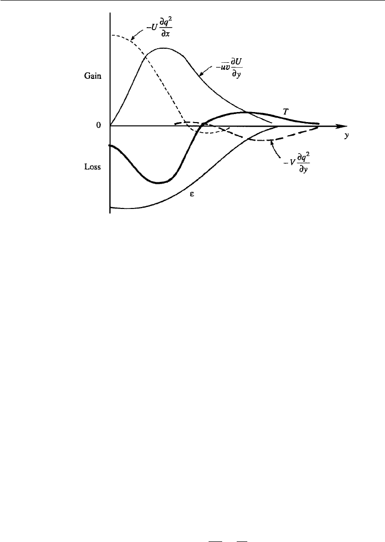
Consider now the kinetic energy budget. For a two-dimensional jet under the

boundary layer assumption ∂/∂x  ∂/∂y, equation (13.34) becomes

0 =−U

∂q

∂x

− V

∂q

∂y

−

∂U

∂y

−

∂

∂y



v + pv/ρ



− ε, (13.46)

where the left-hand side represents ∂q

/∂t = 0. Here the viscous transport and

a term (

− u

)(∂U/∂x) arising out of the shear production have been neglected

on the right-hand side because they are small. The balance of terms is analyzed in

Townsend (1976), and the results are shown in Figure 13.16, where T denotes turbulent

transport represented by the fourth term on the right-hand side of (13.46). The shear

production is zero at the center where both ∂U/∂y and

uv are zero, and reaches a

maximum close to the position of the maximum Reynolds stress. Near the center, the

dissipation is primarily balanced by the downstream advection −U(∂q

/∂x), which is

positive because the turbulent intensity q

decays downstream. Away from the center,

but not too close to the outer edge of the jet, the production and dissipation terms

balance. In the outer parts of the jet, the transport term balances the cross-stream

570 Turbulence

Figure 13.16 Sketch of observed kinetic energy budget in a turbulent jet. Turbulent transport is indi-

cated by T .

advection. In this region V is negative (i.e., toward the center) due to entrainment

of the surrounding ﬂuid, and also q

decreases with y. Therefore the cross-stream

advection −V(∂q

/∂y) is negative, signifying that the entrainment velocity V tends

to decrease the turbulent kinetic energy at the outer edge of the jet. The stationary

state is therefore maintained by the transport term T carrying turbulent kinetic energy

away from the center (where T<0) into the outer parts of the jet (where T>0).

11. Wall-Bounded Shear Flow

The gross characteristics of free shear ﬂows, discussed in the preceding section, are

independent of viscosity. This is not true of a turbulent ﬂow bounded by a solid wall,

in which the presence of viscosity affects the motion near the wall. The effect of

viscosity is reﬂected in the fact that the drag coefﬁcient of a smooth ﬂat plate depends

on the Reynolds number even for Re →∞, as seen in Figure 10.12. Therefore,

the concept of Reynolds number similarity, which says that the gross characteristics

are independent of Re when Re →∞, no longer applies. In this section we shall

examine how the properties of a turbulent ﬂow near a wall are affected by viscosity.

Before doing this, we shall examine how the Reynolds stress should vary with distance

from the wall.

Consider ﬁrst a fully developed turbulent ﬂow in a channel. By “fully developed”

we mean that the ﬂow is no longer changing in x (see Figure 9.2). Then the mean

equation of motion is

0 =−

∂P

∂x

∂ ¯τ

∂y

11. Wall-Bounded Shear Flow 571

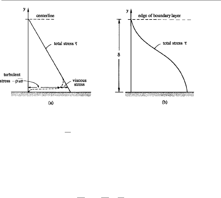
Figure 13.17 Variation of shear stress across a channel and a boundary layer: (a) channel; and (b) boundary

layer.

where ¯τ = µ(dU/dy) − ρ

uv is the total stress. Because ∂P /∂x is a function of x

alone and ∂ ¯τ/∂y is a function of y alone, both of them must be constants. The stress

distribution is then linear (Figure 13.17a). Away from the wall ¯τ is due mostly to the

Reynolds stress, but close to the wall the viscous contribution dominates. In fact, at

the wall the velocity ﬂuctuations and consequently the Reynolds stresses vanish, so

that the stress is entirely viscous.

In a boundary layer on a ﬂat plate there is no pressure gradient and the mean ﬂow

equation is

ρU

∂U

∂x

+ ρV

∂U

∂y

∂ ¯τ

∂y

where ¯τ is a function of x and y. The variation of the stress across a boundary layer

is sketched in Figure 13.17b.

Inner Layer: Law of the Wall

Consider the ﬂow near the wall of a channel, pipe, or boundary layer. Let U

∞

be the

free-stream velocity in a boundary layer or the centerline velocity in a channel and

pipe. Let δ be the width of ﬂow, which may be the width of the boundary layer, the

channel half width, or the radius of the pipe. Assume that the wall is smooth, so that

the height of the surface roughness elements is too small to affect the ﬂow. Physical

considerations suggest that the velocity proﬁle near the wall depends only on the

parameters that are relevant near the wall and does not depend on the free-stream

velocity U

∞

or the thickness of the ﬂow δ. Very near a smooth surface, then, we

expect that

U = U(ρ,τ

,ν,y), (13.47)