Cohen I.M., Kundu P.K. Fluid Mechanics

Подождите немного. Документ загружается.

582 Turbulence

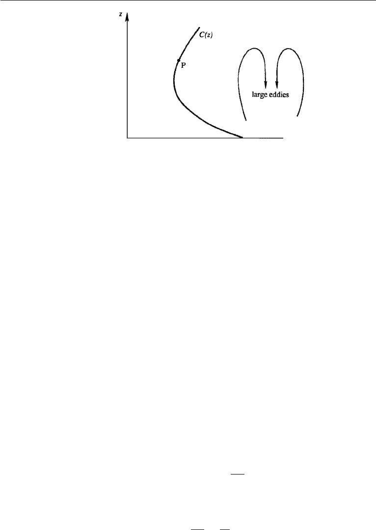
Figure 13.21 An illustration of breakdown of an eddy diffusivity type relation. The eddies are larger than

the scale of curvature of the concentration proﬁle C(z) of carbon monoxide.

In cases where the concept of eddy viscosity may work, we may use the analogy

with equation (13.62), and write

∼ u



, (13.65)

where u



is a typical scale of the ﬂuctuating velocity, and l

is the mixing length,

deﬁned as the cross-stream distance traveled by a ﬂuid particle before it gives up its

momentum and loses identity. The concept of mixing length was ﬁrst introduced by

Taylor (1915), but the approach was fully developed by Prandtl and his coworkers.

As with the eddy viscosity approach, little progress has been made by introducing the

mixing length, because u



and l

are just as unknown as ν

is. Experience shows that

in many situations u



is of the order of either the local mean speed U or the friction

velocity u

∗

. However, there does not seem to be a rational approach for relating l

the mean ﬂow ﬁeld.

Prandtl derived the logarithmic velocity distribution near a solid surface by using

the mixing length theory in the following manner. The scale of velocity ﬂuctuations

in a wall-bounded ﬂow can be taken as u



∼ u

∗

. Prandtl also argued that the mixing

length must be proportional to the distance y. Then equation (13.65) gives

= ku

∗

For points outside the viscous sublayer but still near the wall, the Reynolds stress can

be taken equal to the wall stress ρu

∗

. This gives

ρu

∗

= ρku

∗

which can be written as

∗

. (13.66)

12. Eddy Viscosity and Mixing Length 583

This integrates to

∗

ln y + const.

In recent years the mixing length theory has fallen into disfavor, as it is incorrect

in principle (Tennekes and Lumley, 1972). It only works when there is a single length

scale and a single time scale; for example in the overlap layer in a wall-bounded

ﬂow the only relevant length scale is y and the only time scale is y/u

∗

. However, its

validity is then solely a consequence of dimensional necessity and not of any other

fundamental physics. Indeed it was shown in the preceding section that the loga-

rithmic velocity distribution near a solid surface can be derived from dimensional

considerations alone. (Since u

∗

is the only characteristic velocity in the problem, the

local velocity gradient dU/dy can only be a function of u

∗

and y. This leads to equa-

tion (13.66) merely on dimensional grounds.) Prandtl’s derivation of the empirically

known logarithmic velocity distribution has only historical value.

However, the relationship (13.65) is useful for estimating the order of magnitude

of the eddy diffusivity in a turbulent ﬂow, if we interpret the right-hand side as

simply the product of typical velocity and length scales of large eddies. Consider the

thermal convection between two horizontal plates in air. The walls are separated by

a distance L = 3 m, and the lower layer is warmer by T = 1

◦

C. The equation of

motion (13.33) for the ﬂuctuating ﬁeld gives the vertical acceleration as

∼ gαT



∼

gT

, (13.67)

where we have used the fact that the temperature ﬂuctuations are expected to be of

order T and that α = 1/T for a perfect gas. The time to rise through a height L is

t ∼ L/w, so that equation (13.67) gives a characteristic velocity ﬂuctuation of

w ∼



gLT /T ≈

√

0.1m/s ≈ 0.316 m/s.

It is fair to assume that the largest eddies are as large as the separation between the

plates. The eddy diffusivity is therefore

∼ wL ∼ 0.95 m

/s,

which is much larger than the molecular value of 2 × 10

−5

/s.

As noted in the preceding, the Reynolds averaged Navier–Stokes equations do

not form a closed system. In order for them to be predictive and useful in solving

problems of scientiﬁc and engineering interest, closures must be developed. Reynolds

stresses or higher correlations must be expressed in terms of themselves or lower cor-

relations with empirically determined constants. An excellent review of an important

class of closures is provided by Speziale (1991). Critical discussions of various clo-

sures together with comparisons with each other, with experiments, or with numerical

simulations are given for several idealized problems. Very tragically, Charles Speziale

died while at the peak of his intellectual productivity. He contributed numerous papers

584 Turbulence

on turbulence modeling and other subjects on the foundations of ﬂuid mechanics. A

memorial tribute and a number of papers on turbulence in his honor by some of the

prominent authorities may be found in the May 2006 issue of Journal of Applied

Mechanics (v. 73, no. 3).

A different approach to turbulence modeling is represented by renormalization

group (RNG) theories. Rather than use the Reynolds averaged equations, turbulence

is simulated by a solenoidal isotropic random (body) force ﬁeld f (force/mass). Here

f is chosen to generate the velocity ﬁeld described by the Kolmogorov spectrum in

the limit of large wavenumber K. For very small eddies (larger wavenumbers beyond

the inertial subrange), the energy decays exponentially by viscous dissipation. The

spectrum in Fourier space (K) is truncated at a cutoff wavenumber and the effect

of these very small scales is represented by a modiﬁed viscosity. Then an iteration

is performed successively moving back the cutoff into the inertial range. Smith and

Reynolds (1992) provide a tutorial on the RNG method developed several years

earlier by Yakhot and Orszag. Lam (1992) develops results in a different way and

offers insights and plausible explanations for the various artiﬁces in the theory.

13. Coherent Structures in a Wall Layer

The large-scale identiﬁable structures of turbulent events, called coherent structures,

depend on the type of ﬂow. A possible structure of large eddies found in the outer parts

of a boundary layer, and in a wall-free shear ﬂow, was illustrated in Figure 13.10. In

this section we shall discuss the coherent structures observed within the inner layer

of a wall-bounded shear ﬂow. This is one of the most active areas of current turbulent

research, and reviews of the subject can be found in Cantwell (1981) and Landahl

and Mollo-Christensen (1986).

These structures are deduced from spatial correlation measurements, a certain

amount of imagination, and plenty of ﬂow visualization. The ﬂow visualization

involves the introduction of a marker, one example of which is dye. Another involves

the “hydrogen bubble technique,” in which the marker is generated electrically. A thin

wire is stretched across the ﬂow, and a voltage is applied across it, generating a line

of hydrogen bubbles that travel with the ﬂow. The bubbles produce white spots in the

photographs, and the shapes of the white regions indicate where the ﬂuid is traveling

faster or slower than the average.

Flow visualization experiments by Kline et al. (1967) led to one of the most

important advances in turbulence research. They showed that the inner part of the

wall layer in the range 5 <y

< 70 is not at all passive, as one might think. In fact,

it is perhaps dynamically the most active, in spite of the fact that it occupies only

about 1% of the total thickness of the boundary layer. Figure 13.22 is a photograph

from Kline et al. (1967), showing the top view of the ﬂow within the viscous sublayer

at a distance y

= 2.7 from the wall. (Here x is the direction of ﬂow, and z is the

“spanwise” direction.) The wire producing the hydrogen bubbles in the ﬁgure was

parallel to the z-axis. The streaky structures seen in the ﬁgure are generated by regions

of ﬂuid moving downstream faster or slower than the average. The ﬁgure reveals that

the streaks of low-speed ﬂuid are quasi-periodic in the spanwise direction. From

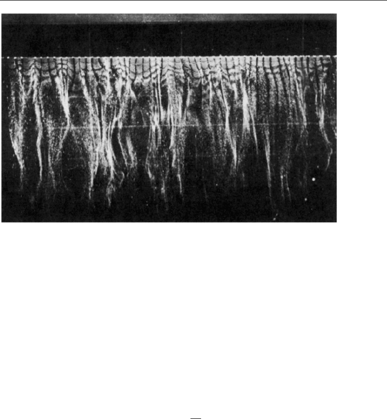
13. Coherent Structures in a Wall Layer 585

Figure 13.22 Top view of near-wall structure (at y

= 2.7) in a turbulent boundary layer on a horizontal

ﬂat plate. The ﬂow is visualized by hydrogen bubbles. S. J. Kline et al., Journal of Fluid Mechanics 30:

741–773, 1967 and reprinted with the permission of Cambridge University Press.

time to time these slowly moving streaks lift up into the buffer region, where they

undergo a characteristic oscillation. The oscillations end violently and abruptly as

the lifted ﬂuid breaks up into small-scale eddies. The whole cycle is called bursting,

or eruption, and is essentially an ejection of slower ﬂuid into the ﬂow above. The

ﬂow into which the ejection occurs decelerates, causing a point of inﬂection in the

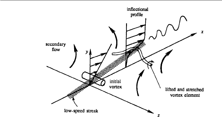
proﬁle u(y) (Figure 13.23). The secondary ﬂow associated with the eruption motion

causes a stretching of the spanwise vortex lines, as sketched in the ﬁgure. These vortex

lines amplify due to the inherent instability of an inﬂectional proﬁle, and readily break

up, producing a source of small-scale turbulence. The strengths of the eruptions vary,

and the stronger ones can go right through to the edge of the boundary layer.

It is clear that the bursting of the slow ﬂuid associates a positive v with a nega-

tive u, generating a positive Reynolds stress −

uv. In fact, measurements show that

most of the Reynolds stress is generated by either the bursting or its counterpart,

called the sweep (or inrush) during which high-speed ﬂuid moves toward the wall.

The Reynolds stress generation is therefore an intermittent process, occurring perhaps

25% of the time.

Largely due to numerical simulations of turbulent ﬂows, it is now understood

that the very large turbulent wall shear stress (as compared with that in laminar

ﬂow) is due to streamwise vorticity in the buffer or inner wall layer (y

= 10–50).

Kim (2003) reports on the history of discovery by computation and experimental

veriﬁcation of insight into the details of turbulent ﬂows. This insight led to strate-

gies to reduce the wall shear stress by active or passive controls. The availability

of microsensors and MEMS actuators creates the possibility of actively modifying

586 Turbulence

Figure 13.23 Mechanics of streak break up. S. J. Kline et al., Journal of Fluid Mechanics 30: 741–773,

1967 and reprinted with the permission of Cambridge University Press.

the ﬂow near the wall to signiﬁcantly reduce the shear stress. Passive modiﬁcation

is exempliﬁed by adding riblets to the surface. These are ﬁne streamwise corruga-

tions that interfere with the interaction between the streamwise vortices and the wall.

Much smaller drag reduction is achieved this way. An example of active modiﬁcation

of the near-wall ﬂow is blowing and suctioning alternately on the surface to counter

the streamwise vorticity. A surprising result of these studies is that linear control

theory (for the Navier–Stokes equation linearized about a mean ﬂow) provides excel-

lent results for a strategy for reducing wall shear stress, provided that function to be

extremized (which cannot be drag) is carefully chosen. All of these results apply only

for small turbulence Reynolds number (Re

∗

= u

∗

δ/ν). However, there has been a

history of success in applying insights gained for small Re

∗

to larger, more realistic

values.

14. Turbulence in a Stratiﬁed Medium

Effects of stratiﬁcation become important in such laboratory ﬂows as heat transfer

from a heated plate and in geophysical ﬂows such as those in the atmosphere and in

the ocean. Some effects of stratiﬁcation on turbulent ﬂows will be considered in this

section. Further discussion can be found in Tennekes and Lumley (1972), Phillips

(1977), and Panofsky and Dutton (1984).

As is customary in geophysical literature, we shall take the z-direction as upward,

and the shear ﬂow will be denoted by U(z). For simplicity the ﬂow will be assumed

homogeneous in the horizontal plane, that is independent of x and y. The turbulence

in a stratiﬁed medium depends critically on the static stability. In the neutrally stable

state of a compressible environment the density decreases upward, because of the

decrease of pressure, at a rate dρ

/dz called the adiabatic density gradient. This

14. Turbulence in a Stratiﬁed Medium 587

is discussed further in Chapter 1, Section 10. A medium is statically stable if the

density decreases faster than the adiabatic decrease. The effective density gradient

that determines the stability of the environment is then determined by the sign of

d(ρ−ρ

)/dz, where ρ −ρ

is called the potential density. In the following discussion,

we shall assume that the adiabatic variations of density have been subtracted out, so

that when we talk about density or temperature, we shall really mean potential density

or potential temperature.

The Richardson Numbers

Let us ﬁrst examine the equation for turbulent kinetic energy (13.34). Omitting the

viscous transport and assuming that the ﬂow is independent of x and y, it reduces to

) =−

∂

∂z



pw + q



−

+ gα



− ε,

where q

= (u

+ v

+ w

)/2. The ﬁrst term on the right-hand side is the transport

of turbulent kinetic energy by ﬂuctuating w. The second term −

uw(dU/dz) is the

production of turbulent energy by the interaction of Reynolds stress and the mean

shear; this term is almost always positive. The third term gα



is the production of

turbulent kinetic energy by the vertical heat ﬂux; it is called the buoyant production,

and was discussed in more detail in Section 7. In an unstable environment, in which

the mean temperature

T decreases upward, the heat ﬂux



is positive (upward),

signifying that the turbulence is generated convectively by upward heat ﬂuxes. In the

opposite case of a stable environment, the turbulence is suppressed by stratiﬁcation.

The ratio of the buoyant destruction of turbulent kinetic energy to the shear production

is called the ﬂux Richardson number:

Rf =

−gα



−uw(dU/dz)

buoyant destruction

shear production

, (13.68)

where we have oriented the x-axis in the direction of ﬂow. As the shear production

is positive, the sign of Rf depends on the sign of



. For an unstable environment

in which the heat ﬂux is upward Rf is negative and for a stable environment it is

positive. For Rf > 1, the buoyant destruction removes turbulence at a rate larger than

the rate at which it is produced by shear production. However, the critical value of Rf

at which the turbulence ceases to be self-supporting is less than unity, as dissipation

is necessarily a large fraction of the shear production. Observations indicate that the

critical value is Rf

 0.25 (Panofsky and Dutton, 1984, p. 94). If measurements

indicate the presence of turbulent ﬂuctuations, but at the same time a value of Rf

much larger than 0.25, then a fair conclusion is that the turbulence is decaying.

When Rf is negative, a large −Rf means strong convection and weak mechanical

turbulence.

Instead of Rf, it is easier to measure the gradient Richardson number, deﬁned as

Ri ≡

(dU/dz)

αg(d

T/dz)

(dU/dz)

, (13.69)

588 Turbulence

where N is the buoyancy frequency. If we make the eddy coefﬁcient assumptions

−



= κ

−

uw = ν

then the two Richardson numbers are related by

Ri =

Rf. (13.70)

The ratio ν

/κ

is the turbulent Prandtl number, which determines the relative efﬁ-

ciency of the vertical turbulent exchanges of momentum and heat. The presence

of a stable stratiﬁcation damps the vertical transports of both heat and momentum;

however, the momentum ﬂux is reduced less because the internal waves in a sta-

ble environment can transfer momentum (by moving vertically from one region to

another) but not heat. Therefore, ν

/κ

> 1 for a stable environment. Equation (13.70)

then shows that turbulence can persist even when Ri > 1, if the critical value of 0.25

applies on the ﬂux Richardson number (Turner, 1981; Bradshaw and Woods, 1978).

In an unstable environment, on the other hand, ν

/κ

becomes small. In a neutral envi-

ronment it is usually found that ν

 κ

; the idea of equating the eddy coefﬁcients of

heat and momentum is called the Reynolds analogy.

Monin–Obukhov Length

The Richardson numbers are ratios that compare the relative importance of mechanical

and convective turbulence. Another parameter used for the same purpose is not a ratio,

but has the unit of length. It is the Monin–Obukhov length, deﬁned as

≡−

∗

kαgwT



, (13.71)

where u

∗

is the friction velocity, wT



is the heat ﬂux, α is the coefﬁcient of thermal

expansion, and k is the von Karman constant introduced for convenience. Although



is a function of z, the parameter L

is effectively a constant for the ﬂow, as

it is used only in the logarithmic surface layer in which both the stress and the

heat ﬂux



are nearly constant. The Monin–Obukhov length then becomes a

parameter determined from the boundary conditions of drag and the heat ﬂux at

the surface. Like Rf, it is positive for stable conditions and negative for unstable

conditions.

The signiﬁcance of L

within the surface layer becomes clearer if we write

Rf in terms of L

, using the logarithmic velocity distribution (13.60), from which

dU/dz = u

∗

/kz. (Note that we are now using z for distances perpendicular to the

surface.) Using

uw = u

∗

because of the near uniformity of stress in the logarithmic

14. Turbulence in a Stratiﬁed Medium 589

layer, equation (13.68) becomes

Rf =

. (13.72)

As Rf is the ratio of buoyant destruction to shear production of turbulence, (13.72)

shows that L

is the height at which these two effects are of the same order.

For both stable and unstable conditions, the effects of stratiﬁcation are slight if

z |L

|. At these small heights, then, the velocity proﬁle is logarithmic, as in a

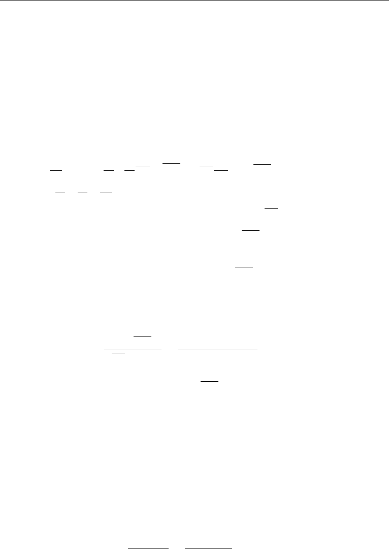
neutral environment. This is called a forced convection region, because the turbu-

lence is mechanically forced. For z |L

|, the effects of stratiﬁcation dominate.

In an unstable environment, it follows that the turbulence is generated mainly by

buoyancy at heights z −L

, and the shear production is negligible. The region

beyond the forced convecting layer is therefore called a zone of free convection

(Figure 13.24), containing thermal plumes (columns of hot rising gases) characteristic

of free convection from heated plates in the absence of shear ﬂow.

Observations as well as analysis show that the effect of stratiﬁcation on the veloc-

ity distribution in the surface layer is given by the log-linear proﬁle (Turner, 1973)

U =

∗



+ 5



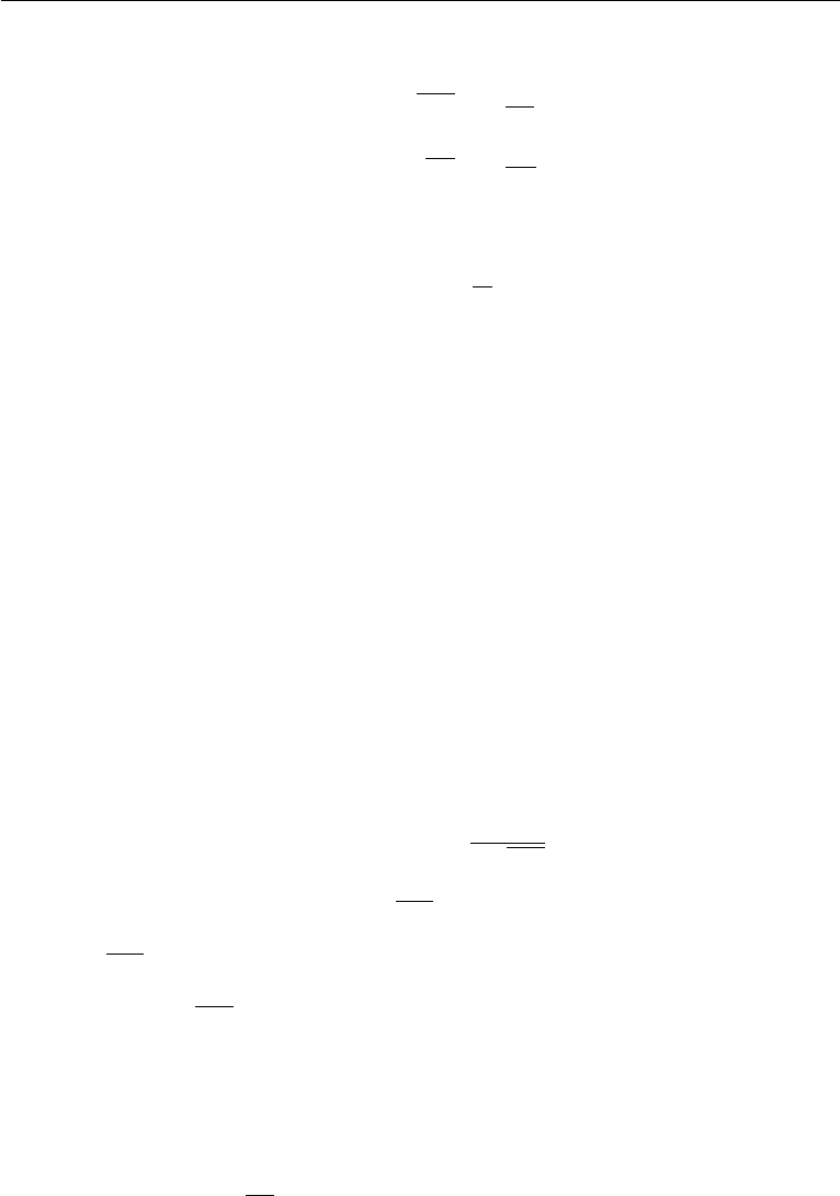
The form of this proﬁle is sketched in Figure 13.25 for stable and unstable conditions.

It shows that the velocity is more uniform than ln z in the unstable case because of

the enhanced vertical mixing due to buoyant convection.

Spectrum of Temperature Fluctuations

An equation for the intensity of temperature ﬂuctuations

2

can be obtained in a

manner identical to that used for obtaining the turbulent kinetic energy. The procedure

is therefore to obtain an equation for DT



/Dt by subtracting those for D

T/Dt and

Figure 13.24 Forced and free convection zones in an unstable atmosphere.

590 Turbulence

Figure 13.25 Effect of stability on velocity proﬁles in the surface layer.

T/Dt, and then to multiply the resulting equation for DT



/Dt by T



and take the

average. The result is

2

=−



−

∂

∂z



2

w − κ

2



− ε

where ε

≡ κ(∂T



/∂x

)

is the dissipation of temperature ﬂuctuation, analogous

to the dissipation of turbulent kinetic energy ε = 2ν

. The ﬁrst term on the

right-hand side is the generation of

2

by the mean temperature gradient, wT



being

positive if d

T/dzis negative. The second term on the right-hand side is the turbulent

transport of

2

A wavenumber spectrum of temperature ﬂuctuations can be deﬁned such that

2

≡



∞

(K) dK.

As in the case of the kinetic energy spectrum, an inertial range of wavenumbers

exists in which neither the production by large-scale eddies nor the dissipation by

conductive and viscous effects are important. As the temperature ﬂuctuations are

intimately associated with velocity ﬂuctuations, (K) in this range must depend not

only on ε

but also on the variables that determine the velocity spectrum, namely ε

and K. Therefore

(K) = (ε

,ε,K) l

−1

 K  η

−1

15. Taylor’s Theory of Turbulent Dispersion 591

The unit of  is

◦

m, and the unit of ε

◦

/s. A dimensional analysis gives

(K) ∝ ε

−1/3

−5/3

−1

 K  η

−1

, (13.73)

which was ﬁrst derived by Obukhov in 1949. Comparing with equation (13.40), it is

apparent that the spectra of both velocity and temperature ﬂuctuations in the inertial

subrange have the same K

−5/3

form.

The spectrum beyond the inertial subrange depends on whether the Prandtl num-

ber ν/κ of the ﬂuid is smaller or larger than one. We shall only consider the case of

ν/κ  1, which applies to water for which the Prandtl number is 7.1. Let η

be the

scale responsible for smearing out the temperature gradients and η be the Kolmogorov

microscale at which the velocity gradients are smeared out. For ν/κ  1 we expect

that η

 η, because then the conductive effects are important at scales smaller than

the viscous scales. In fact, Batchelor (1959) showed that η

 η(κ/ν)

1/2

 η.In

such a case there exists a range of wavenumbers η

−1

 K  η

−1

, in which the

scales are not small enough for the thermal diffusivity to smear out the temperature

ﬂuctuation. Therefore, (K) continues farther up to η

−1

, although S(K) drops off

sharply. This is called the viscous convective subrange, because the spectrum is dom-

inated by viscosity but is still actively convective. Batchelor (1959) showed that the

spectrum in the viscous convective subrange is

(K) ∝ K

−1

 K  η

−1

. (13.74)

Figure 13.26 shows a comparison of velocity and temperature spectra, observed in a

tidal ﬂow through a narrow channel. The temperature spectrum shows that the spectral

slope increases from −

in the inertial subrange to −1 in the viscous convective

subrange.

15. Taylor’s Theory of Turbulent Dispersion

The large mixing rate in a turbulent ﬂow is due to the fact that the ﬂuid particles

gradually wander away from their initial location. Taylor (1921) studied this problem

and calculated the rate at which a particle disperses (i.e., moves away) from its initial

location. The presentation here is directly adapted from his classic paper. He consid-

ered a point source emitting particles, say a chimney emitting smoke. The particles

are emitted into a stationary and homogeneous turbulent medium in which the mean

velocity is zero. Taylor used Lagrangian coordinates X(a,t), which is the present

location at time t of a particle that was at location a at time t = 0. We shall take the

point source to be the origin of coordinates and consider an ensemble of experiments

in which we measure the location X(0,t) at time t of all the particles that started

from the origin (Figure 13.27). For simplicity we shall suppress the ﬁrst argument in

X(0,t)and write X(t) to mean the same thing.

Rate of Dispersion of a Single Particle

Consider the behavior of a single component of X, say X

(α = 1, 2, or 3). (We are

using a Greek subscript α because we shall not imply the summation convention.)