Cohen I.M., Kundu P.K. Fluid Mechanics

Подождите немного. Документ загружается.

252 Gravity Waves

Finite Amplitude Waves in Fairly Shallow Water: Solitons

Next, consider nonlinear waves in a slightly dispersive system, such as “fairly long”

waves with λ/H in the range between 10 and 20. In 1895 Korteweg and deVries

showed that these waves approximately satisfy the nonlinear equation

∂η

∂t

+ c

∂η

∂x

∂η

∂x

∂

∂x

= 0, (7.92)

where c

√

gH. This is the Korteweg–deVries equation. The ﬁrst two terms appear

in the linear nondispersive limit. The third term is due to ﬁnite amplitude effects and

the fourth term results from the weak dispersion due to the water depth being not

shallow enough. (Neglecting the nonlinear term in equation (7.92), and substituting

η = a exp(ikx − iωt), it is easy to show that the dispersion relation is c = c

(1 −

(1/6)k

). This agrees with the ﬁrst two terms in the Taylor series expansion of the

dispersion relation c =

√

(g/k) tanh kH for small kH, verifying that weak dispersive

effects are indeed properly accounted for by the last term in equation (7.92).)

The ratio of nonlinear and dispersion terms in equation (7.92) is

∂η

∂x



∂

∂x

∼

aλ

When aλ

is larger than ≈16, nonlinear effects sharpen the forward face of

the wave, leading to hydraulic jump, as discussed in Section 11. For lower values

of aλ

, a balance can be achieved between nonlinear steepening and disper-

sive spreading, and waves of unchanging form become possible. Analysis of the

Korteweg–deVries equation shows that two types of solutions are then possible, a

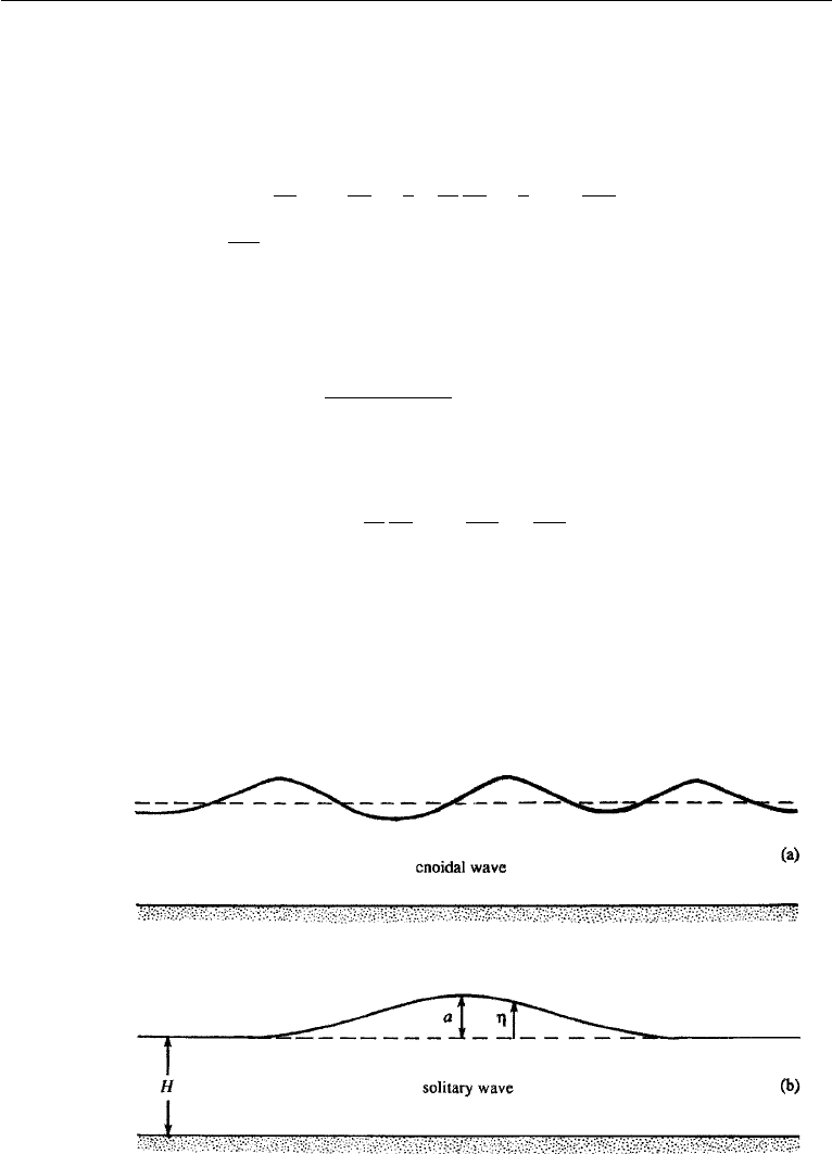
periodic solution and a solitary wave solution. The periodic solution is called cnoidal

Figure 7.25 Cnoidal and solitary waves. Waves of unchanging form result because nonlinear steepening

balances dispersive spreading.

14. Stokes’ Drift 253

wave, because it is expressed in terms of elliptic functions denoted by cn(x). Its wave-

form is shown in Figure 7.25. The other possible solution of the Korteweg–deVries

equation involves only a single hump and is called a solitary wave or soliton. Its

proﬁle is given by

η = a sech







1/2

(x − ct)



, (7.93)

where the speed of propagation is

c = c



1 +



showing that the propagation velocity increases with the amplitude of the hump. The

validity of equation (7.93) can be checked by substitution into equation (7.92). The

waveform of the solitary wave is shown in Figure 7.25.

An isolated hump propagating at constant speed with unchanging form and in

fairly shallow water was ﬁrst observed experimentally by S. Russell in 1844. Soli-

tons have been observed to exist not only as surface waves, but also as internal

waves in stratiﬁed ﬂuid, in the laboratory as well as in the ocean; (See Figure 3.3,

Turner (1973)).

14. Stokes’ Drift

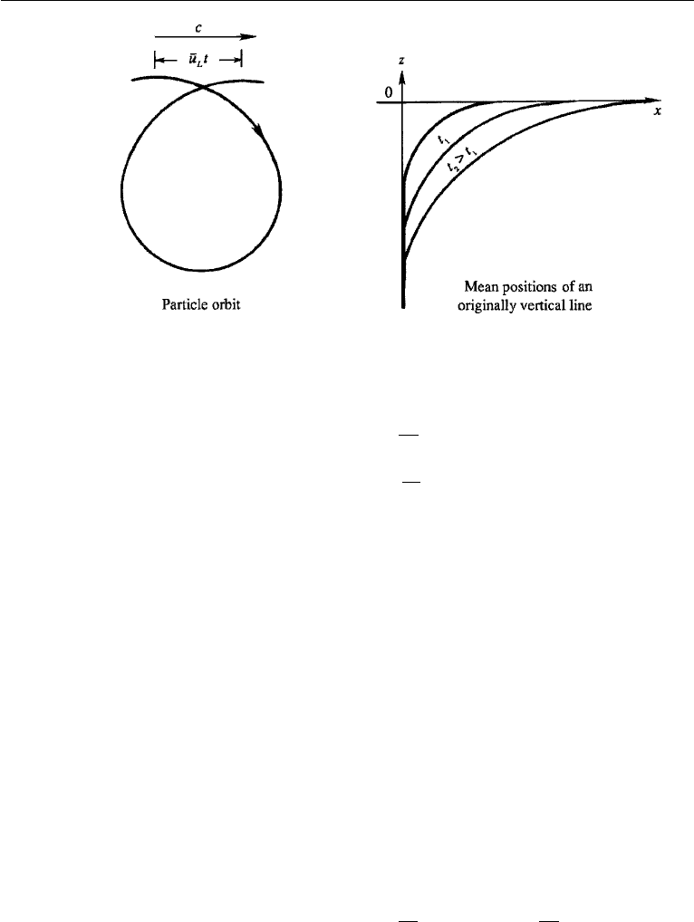
Anyone who has observed the motion of a ﬂoating particle on the sea surface knows

that the particle moves slowly in the direction of propagation of the waves. This is

called Stokes’ drift. It is a second-order or ﬁnite amplitude effect, due to which the

particle orbit is not closed but has the shape shown in Figure 7.26. The mean velocity

of a ﬂuid particle (that is, the Lagrangian velocity) is therefore not zero, although

the mean velocity at a point (the Eulerian velocity) must be zero if the process is

periodic. The drift is essentially due to the fact that the particle moves forward faster

(when it is at the top of its trajectory) than backward (when it is at the bottom of its

orbit). Although it is a second-order effect, its magnitude is frequently signiﬁcant.

To ﬁnd an expression for Stokes’ drift, we use Lagrangian speciﬁcation, proceed-

ing as in Section 5 but keeping a higher order of accuracy in the analysis. Our analysis

is adapted from the presentation given in the work by Phillips (1977, p. 43). Let (x, z)

be the instantaneous coordinates of a ﬂuid particle whose position at t = 0is(x

The initial coordinates (x

) serve as a particle identiﬁcation, and we can write

its subsequent position as x(x

,t) and z(x

,t), using the Lagrangian form of

speciﬁcation. The velocity components of the “particle (x

)” are u

,t)and

,t). (Note that the subscript “L” was not introduced in Section 5, since to

the lowest order we equated the velocity at time t of a particle with mean coordinates

) to the Eulerian velocity at t at location (x

). Here we are taking the analy-

sis to a higher order of accuracy, and the use of a subscript “L” to denote Lagrangian

velocity helps to avoid confusion.)

254 Gravity Waves

Figure 7.26 The Stokes drift.

The velocity components are

∂x

∂t

∂z

∂t

(7.94)

where the partial derivative signs mean that the initial position (serving as a particle

tag) is kept ﬁxed in the time derivative. The position of a particle is found by integrating

equation (7.94):

x = x





)dt



z = z





)dt



(7.95)

At time t the Eulerian velocity at (x, z) equals the Lagrangian velocity of particle

) at the same time, if (x, z) and (x

) are related by equation (7.95). (No

approximation is involved here! The equality is merely a reﬂection of the fact that

particle (x

) occupies the position (x,z) at time t.) Denoting the Eulerian velocity

components without subscript, we therefore have

,t) = u(x, z, t ).

Expanding the Eulerian velocity u(x,z,t)in a Taylor series about (x

), we obtain

,t) = u(x

,t)+ (x − x

)



∂u

∂x



+ (z − z

)



∂u

∂z



+···, (7.96)

and a similar expression for w

. The Stokes drift is the time mean value of equa-

tion (7.96). As the time mean of the ﬁrst term on the right-hand side of equation (7.96)

15. Waves at a Density Interface between Inﬁnitely Deep Fluids 255

is zero, the Stokes drift is given by the mean of the next two terms of equation (7.96).

This was neglected in Section 5, and the result was closed orbits.

We shall now estimate the Stokes drift for gravity waves, using the deep water

approximation for algebraic simplicity. The velocity components and particle dis-

placements for this motion are given in Section 6 as

u(x

,t) = aωe

cos(kx

− ωt),

x − x

=−ae

sin(kx

− ωt),

z − z

= ae

cos(kx

− ωt).

Substitution into the right-hand side of equation (7.96), taking time average, and using

the fact that the time average of sin

t over a time period is 1/2, we obtain

¯u

= a

ωke

2kz

, (7.97)

which is the Stokes drift in deep water. Its surface value is a

ωk, and the vertical

decay rate is twice that for the Eulerian velocity components. It is therefore conﬁned

very close to the sea surface. For arbitrary water depth, it is easy to show that

¯u

= a

ωk

cosh 2k(z

+ H)

2 sinh

. (7.98)

The Stokes drift causes mass transport in the ﬂuid, due to which it is also called

the mass transport velocity. Vertical ﬂuid lines marked, for example, by some dye

gradually bend over (Figure 7.26). In spite of this mass transport, the mean Eulerian

velocity anywhere below the trough is exactly zero (to any order of accuracy), if the

ﬂow is irrotational. This follows from the condition of irrotationality ∂u/∂z = ∂w/∂x,

a vertical integral of which gives

u = u|

z=−H



−H

∂w

∂x

dz,

showing that the mean of u is proportional to the mean of ∂w/∂x over a wavelength,

which is zero for periodic ﬂows.

15. Waves at a Density Interface between Inﬁnitely Deep Fluids

To this point we have considered only waves at the free surface of a liquid. However,

waves can also exist at the interface between two immiscible liquids of different

densities. Such a sharp density gradient can, for example, be generated in the ocean

by solar heating of the upper layer, or in an estuary (that is, a river mouth) or a fjord into

which fresh (less saline) river water ﬂows over oceanic water, which is more saline

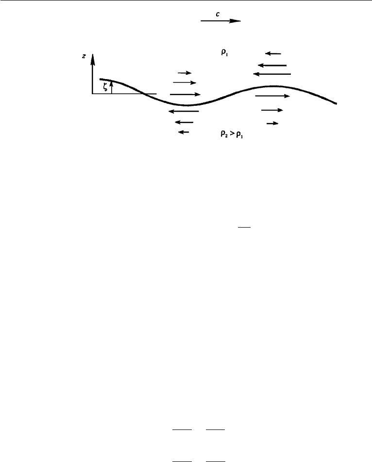
and consequently heavier. The situation can be idealized by considering a lighter ﬂuid

of density ρ

lying over a heavier ﬂuid of density ρ

(Figure 7.27).

We assume that the ﬂuids are inﬁnitely deep, so that only those solutions that

decay exponentially from the interface are allowed. In this section and in the rest of

256 Gravity Waves

Figure 7.27 Internal wave at a density interface between two inﬁnitely deep ﬂuids.

the chapter, we shall make use of the convenience of complex notation. For example,

we shall represent the interface displacement ζ = a cos(kx − ωt) by

ζ = Reae

i(kx−ωt)

where Re stands for “the real part of,” and i =

√

−1. It is customary to omit the Re

symbol and simply write

ζ = ae

i(kx−ωt)

, (7.99)

where it is implied that only the real part of the equation is meant. We are therefore

carrying an extra imaginary part (which can be thought of as having no physical

meaning) on the right-hand side of equation (7.99). The convenience of complex

notation is that the algebra is simpliﬁed, essentially because differentiating expo-

nentials is easier than differentiating trigonometric functions. If desired, the con-

stant a in equation (7.99) can be considered to be a complex number. For example,

the proﬁle ζ = sin(kx − ωt) can be represented as the real part of ζ =−i exp

i(kx − ωt).

We have to solve the Laplace equation for the velocity potential in both lay-

ers, subject to the continuity of p and w at the interface. The equations are,

therefore,

∂

∂x

∂

∂z

= 0

∂

∂x

∂

∂z

= 0,

(7.100)

subject to

→0asz →∞ (7.101)

→0asz →−∞ (7.102)

15. Waves at a Density Interface between Inﬁnitely Deep Fluids 257

∂φ

∂z

∂φ

∂z

∂ζ

∂t

at z = 0 (7.103)

∂φ

∂t

+ ρ

gζ =ρ

∂φ

∂t

+ ρ

gζ at z = 0. (7.104)

Equation (7.103) follows from equating the vertical velocity of the ﬂuid on both

sides of the interface to the rate of rise of the interface. Equation (7.104) follows

from the continuity of pressure across the interface. As in the case of surface waves,

the boundary conditions are linearized and applied at z = 0 instead of at z = ζ .

Conditions (7.101) and (7.102) require that the solutions of equation (7.100) must be

of the form

= Ae

−kz

i(kx−ωt)

= Be

i(kx−ωt)

because a solution proportional to e

is not allowed in the upper ﬂuid, and a solution

proportional to e

−kz

is not allowed in the lower ﬂuid. Here A and B can be complex.

As in Section 4, the constants are determined from the kinematic boundary conditions

(7.103), giving

A =−B = iωa/k.

The dynamic boundary condition (7.104) then gives the dispersion relation

ω =





− ρ

+ ρ



= ε



gk, (7.105)

where ε

≡ (ρ

−ρ

)/(ρ

+ρ

) is a small number if the density difference between

the two liquids is small. The case of small density difference is relevant in geophysical

situations; for example, a 10

◦

C temperature change causes the density of the upper

layer of the ocean to decrease by 0.3%. Equation (7.105) shows that waves at the

interface between two liquids of inﬁnite thickness travel like deep water surface

waves, with ω proportional to

√

gk, but at a much reduced frequency. In general,

therefore, internal waves have a smaller frequency, and consequently a smaller phase

speed, than surface waves. As expected, equation (7.105) reduces to the expression

for surface waves if ρ

= 0.

The kinetic energy of the ﬁeld can be found by integrating ρ(u

+ w

)/2 over

the range z =±∞. This gives the average kinetic energy per unit horizontal area of

(see Exercise 7):

(ρ

− ρ

)ga

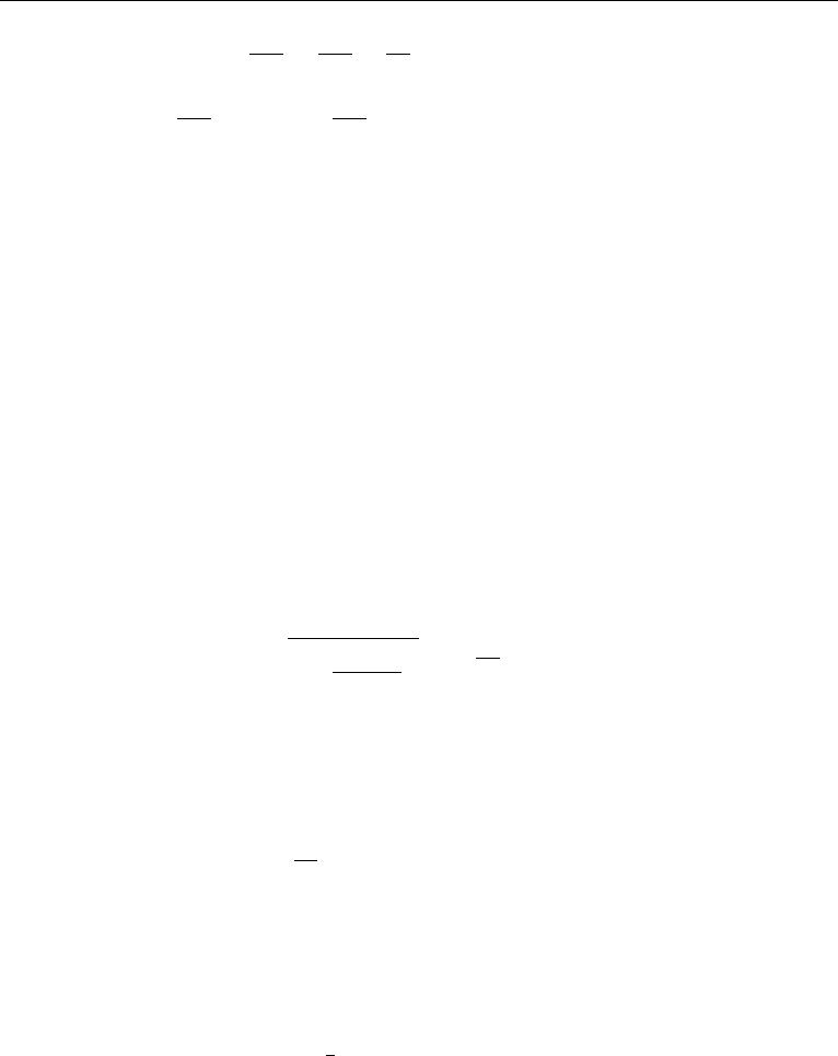
The potential energy can be calculated by ﬁnding the rate of work done in deforming

a ﬂat interface to the wave shape. In Figure 7.28, this involves a transfer of column

A of density ρ

to location B, a simultaneous transfer of column B of density ρ

to location A, and integrating the work over half the wavelength, since the resulting

258 Gravity Waves

Figure 7.28 Calculation of potential energy of a two-layer ﬂuid. The work done in transferring element

A to B equals the weight of A times the vertical displacement of its center of gravity.

exchange forms a complete wavelength; see the previous discussion of Figure 7.8.

The potential energy per unit horizontal area is therefore



λ/2

gζ

dx −



λ/2

gζ

g(ρ

− ρ

)

2λ



λ/2

dx =

(ρ

− ρ

)ga

The total wave energy per unit horizontal area is

E = E

+ E

(ρ

− ρ

)ga

. (7.106)

In a comparison with equation (7.55), it follows that the amplitude of internal waves

is usually much larger than those of surface waves if the same amount of energy is

used to set off the motion.

The horizontal velocity components in the two layers are

∂φ

∂x

=−ωae

−kz

i(kx−ωt)

∂φ

∂x

= ωae

i(kx−ωt)

which show that the velocities in the two layers are oppositely directed (Figure 7.27).

The interface is therefore a vortex sheet, which is a surface across which the tangential

velocity is discontinuous. It can be expected that a continuously stratiﬁed medium, in

which the density varies continuously as a function of z, will support internal waves

whose vorticity is distributed throughout the ﬂow. Consequently, internal waves in

a continuously stratiﬁed ﬂuid are not irrotational and do not satisfy the Laplace

equation. This is discussed further in Section 16.

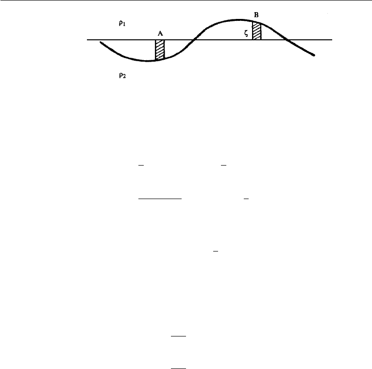
The existence of internal waves at a density discontinuity has explained an inter-

esting phenomenon observed in Norwegian fjords (Gill, 1982). It was known for a

long time that ships experienced unusually high drags on entering these fjords. The

phenomenon was a mystery (and was attributed to “dead water”!) until Bjerknes, a

Norwegian oceanographer, explained it as due to the internal waves at the interface

generated by the motion of the ship (Figure 7.29). (Note that the product of the drag

16. Waves in a Finite Layer Overlying an Inﬁnitely Deep Fluid 259

Figure 7.29 Phenomenon of “dead water” in Norwegian fjords.

times the speed of the ship gives the rate of generation of wave energy, with other

sources of resistance neglected.)

16. Waves in a Finite Layer Overlying an Inﬁnitely Deep Fluid

As a second example of an internal wave at a density discontinuity, consider the case

in which the upper layer is not inﬁnitely thick but has a ﬁnite thickness; the lower

layer is initially assumed to be inﬁnitely thick. The case of two inﬁnitely deep liquids,

treated in the preceding section, is then a special case of the present situation. Whereas

only waves at the interface were allowed in the preceding section, the presence of the

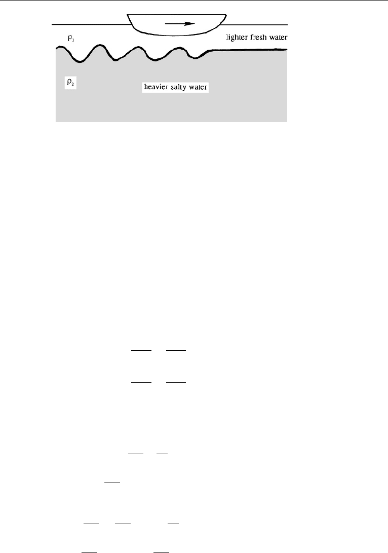
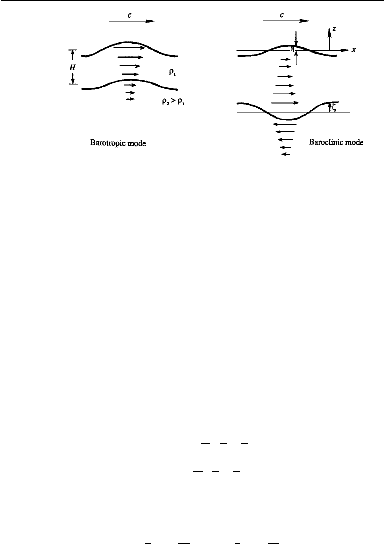
free surface now allows an extra mode of surface waves. It is clear that the present

conﬁguration will allow two modes of oscillation, one in which the free surface and

the interface are in phase and a second mode in which they are oppositely directed.

Let H be the thickness of the upper layer, and let the origin be placed at the mean

position of the free surface (Figure 7.30). The equations are

∂

∂x

∂

∂z

= 0

∂

∂x

∂

∂z

= 0,

subject to

→ 0atz →−∞ (7.107)

∂φ

∂z

∂η

∂t

at z = 0 (7.108)

∂φ

∂t

+ gη = 0atz = 0 (7.109)

∂φ

∂z

∂φ

∂z

∂ζ

∂t

at z =−H (7.110)

∂φ

∂t

+ ρ

gζ =ρ

∂φ

∂t

+ ρ

gζ at z =−H. (7.111)

260 Gravity Waves

Figure 7.30 Two modes of motion of a layer of ﬂuid overlying an inﬁnitely deep ﬂuid.

Assume a free surface displacement of the form

η = ae

i(kx−ωt)

, (7.112)

and an interface displacement of the form

ζ = be

i(kx−ωt)

. (7.113)

As before, only the real part of the right-hand side is meant. Without losing generality,

we can regard a as real, which means that we are considering a wave of the form

η = a cos(kx − ωt). The constant b should be left complex, because ζ and η may

not be in phase. Solution of the problem determines such phase differences.

The velocity potentials in the layers must be of the form

= (A e

+ Be

−kz

i(kx−ωt)

, (7.114)

= Ce

i(kx−ωt)

. (7.115)

The form (7.115) is chosen in order to satisfy equation (7.107). Conditions

(7.108)–(7.110) give the constants in terms of the given amplitude a:

A =−





, (7.116)

B =



−



, (7.117)

C =−





−



−



2kH

, (7.118)

b =



1 +



−kH



1 −



. (7.119)

16. Waves in a Finite Layer Overlying an Inﬁnitely Deep Fluid 261

Substitution into equation (7.111) gives the required dispersion relation ω(k). After

some algebraic manipulations, the result can be written as (Exercise 8)



− 1



[ρ

sinh kH + ρ

cosh kH]−(ρ

− ρ

) sinh kH



= 0. (7.120)

The two possible roots of this equation are discussed in what follows.

Barotropic or Surface Mode

One possible root of equation (7.120) is

= gk, (7.121)

which is the same as that for a deep water gravity wave. Equation (7.119) shows that

in this case

b = ae

−kH

, (7.122)

implying that the amplitude at the interface is reduced from that at the surface by the

factor e

−kH

. Equation (7.122) also shows that the motions of the interface and the

free surface are locked in phase; that is they go up or down simultaneously. This mode

is similar to a gravity wave propagating on the free surface of the upper liquid, in

which the motion decays as e

−kz

from the free surface. It is called the barotropic

mode, because the surfaces of constant pressure and density coincide in such

aﬂow.

Baroclinic or Internal Mode

The other possible root of equation (7.120) is

gk(ρ

− ρ

) sinh kH

cosh kH + ρ

sinh kH

, (7.123)

which reduces to equation (7.105) if kH →∞. Substitution of equation (7.123) into

(7.119) shows that, after some straightforward algebra,

η =−ζ



− ρ



−kH

, (7.124)

demonstrating that η and ζ have opposite signs and that the interface displacement

is much larger than the surface displacement if the density difference is small. This

mode of behavior is called the baroclinic or internal mode because the surfaces of

constant pressure and density do not coincide. It can be shown that the horizontal

velocity u changes sign across the interface. The existence of a density difference has

therefore generated a motion that is quite different from the barotropic behavior. The

case studied in the previous section, in which the ﬂuids have inﬁnite depth and no

free surface, has only a baroclinic mode and no barotropic mode.