Cohen I.M., Kundu P.K. Fluid Mechanics

Подождите немного. Документ загружается.

202 Irrotational Flow

If, however, the ﬂow is symmetrical about axis, one of the streamfunctions is known

because all streamlines must lie in planes passing through the axis of symmetry. In

cylindrical polar coordinates, one streamfunction, say, χ, may be taken as χ =−ϕ.

In spherical polar coordinates (see Figure 6.27), the choice χ =−ϕ is also appro-

priate if all streamlines are in ϕ = const. planes through the axis of symmetry. Then

ρu = ∇χ × ∇ψ. We shall see that the streamfunction for these axisymmetric ﬂows

does not satisfy the Laplace equation (and consequently the method of complex vari-

ables is not applicable) and the lines of constant φ and ψ are not orthogonal. Some

simple examples of axisymmetric irrotational ﬂows around bodies of revolution, such

as spheres and airships, will be given in the rest of this chapter.

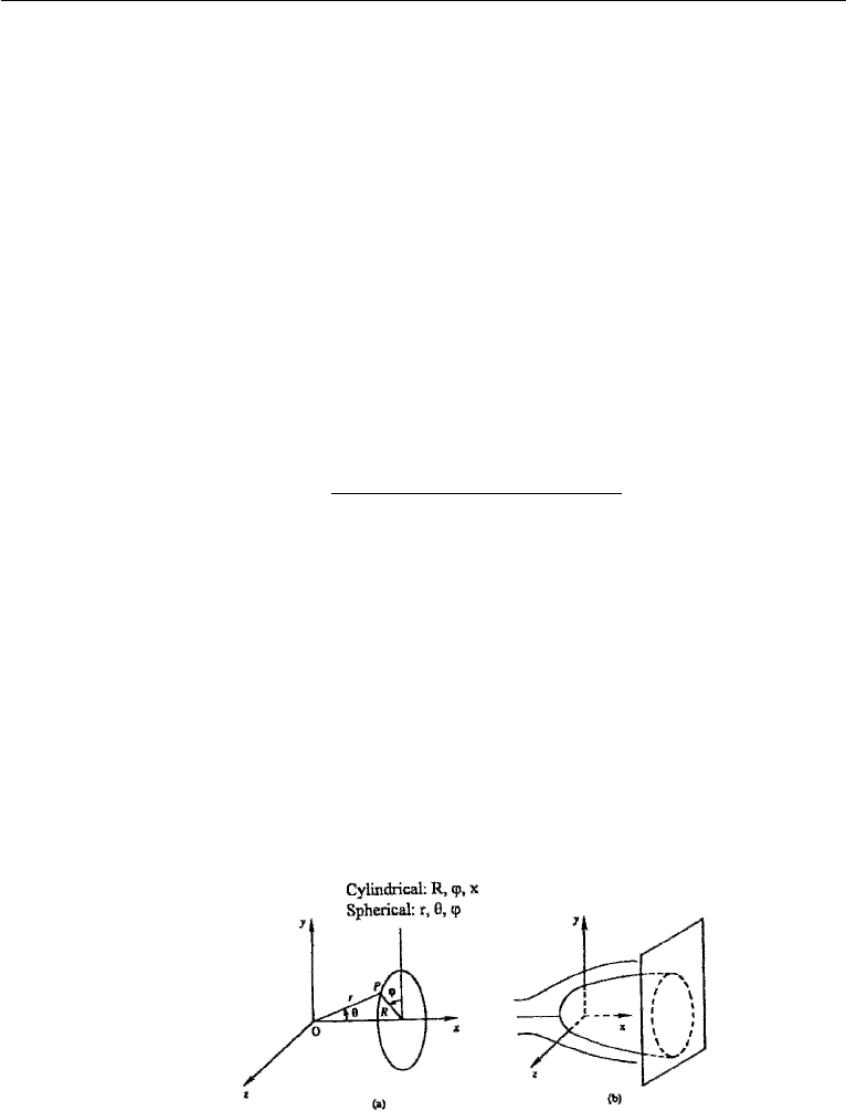
In axisymmetric ﬂow problems, it is convenient to work with both cylindrical

and spherical polar coordinates, often going from one set to the other in the same

problem. In this chapter cylindrical coordinates will be denoted by (R, ϕ, x), and

spherical coordinates by (r, θ , ϕ). These are illustrated in Figure 6.27a, from which

their relation to Cartesian coordinates is seen to be

cylindrical spherical

x = xx= r cos θ

y = R cos ϕy= r sin θ cos ϕ

z = R sin ϕz= r sin θ sin ϕ

(6.63)

Note that r is the distance from the origin, whereas R is the radial distance from

the x-axis. The bodies of revolution will have their axes coinciding with the x-axis

(Figure 6.27b). The resulting ﬂow pattern is independent of the azimuthal coordinate

ϕ, and is identical in all planes containing the x-axis. Further, the velocity component

is zero.

Important expressions for curvilinear coordinates are listed in Appendix B. For

axisymmetric ﬂows, several relevant expressions are presented in the following for

quick reference.

Figure 6.27 (a) Cylindrical and spherical coordinates; (b) axisymmetric ﬂow. In Fig. 6.27, the coor-

dinate axes are not aligned according to the conventional deﬁnitions. Speciﬁcally in (a), the polar axis

from which θ is measured is usually taken to be the z-axis and ϕ is measured from the x-axis. In

(b), the axis of symmetry is usually taken to be the z-axis and the angle θ or ϕ is measured from the

x-axis.

18. Streamfunction and Velocity Potential for Axisymmetric Flow 203

Continuity equation:

∂u

∂x

∂

∂R

(Ru

) = 0 (cylindrical) (6.64)

∂

∂r

) +

sin θ

∂

∂θ

sin θ) = 0 (spherical) (6.65)

Laplace equation:

∇

φ =

∂

∂R



∂φ

∂R



∂

∂x

= 0 (cylindrical) (6.66)

∇

φ =



∂

∂r



∂φ

∂r



sin θ

∂

∂θ



sin θ

∂φ

∂θ



= 0 (spherical) (6.67)

Vorticity:

∂u

∂x

−

∂u

∂R

(cylindrical) (6.68)



∂

∂r

(ru

) −

∂u

∂θ



(spherical) (6.69)

18. Streamfunction and Velocity Potential for

Axisymmetric Flow

A streamfunction can be deﬁned for axisymmetric ﬂows because the continuity equa-

tion involves two terms only. In cylindrical coordinates, the continuity equation can

be written as

∂

∂x

(Ru

) +

∂

∂R

(Ru

) = 0 (6.70)

which is satisﬁed by u =−∇ϕ × ∇ψ , yielding

≡

∂ψ

∂R

(cylindrical),

≡−

∂ψ

∂x

(6.71)

The axisymmetric stream function is sometimes called the Stokes streamfunction.It

has units of m

/s, in contrast to the streamfunction for plane ﬂow, which has units of

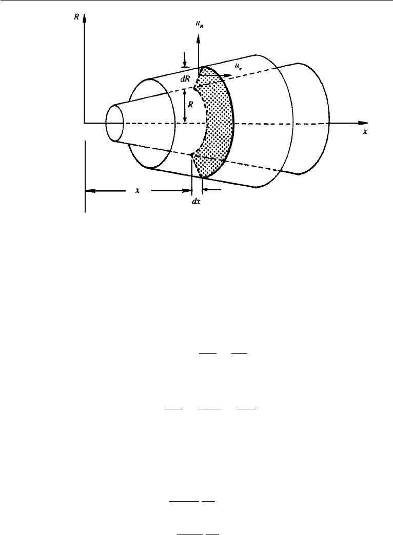
/s. Due to the symmetry of ﬂow about the x-axis, constant ψ surfaces are surfaces

of revolution. Consider two streamsurfaces described by constant values of ψ and

ψ +dψ (Figure 6.28). The volumetric ﬂow rate through the annular space is

dQ =−u

(2πR dx) + u

(2πR d R) = 2π



∂ψ

∂x

dx +

∂ψ

∂R



= 2πdψ,

204 Irrotational Flow

Figure 6.28 Axisymmetric streamfunction. The volume ﬂow rate through two streamsurfaces is 2πψ.

where equation (6.71) has been used. The form dψ = dQ/2π shows that the differ-

ence in ψ values is the ﬂow rate between two concentric streamsurfaces per unit radian

angle around the axis. This is consistent with the extended discussion of streamfunc-

tions in Chapter 4, Section 4. The factor of 2π is absent in plane two-dimensional

ﬂows, where dψ = dQis the ﬂow rate per unit depth. The sign convention is the same

as for plane ﬂows, namely, that ψ increases toward the left if we look downstream.

If the ﬂow is also irrotational, then

∂u

∂x

−

∂u

∂R

= 0. (6.72)

On substituting equation (6.71) into equation (6.72), we obtain

∂

∂R

−

∂ψ

∂R

∂

∂x

= 0, (6.73)

which is different from the Laplace equation (6.66) satisﬁed by φ. It is easy to show

that lines of constant φ and ψ are not orthogonal. This is a basic difference between

axisymmetric and plane ﬂows.

In spherical coordinates, the streamfunction is deﬁned as u =−∇ϕ × ∇ψ,

yielding

sin θ

∂ψ

∂θ

(spherical),

=−

r sin θ

∂ψ

∂r

(6.74)

which satisﬁes the axisymmetric continuity equation (6.65).

19. Simple Examples of Axisymmetric Flows 205

The velocity potential for axisymmetric ﬂow is deﬁned as

cylindrical spherical

∂φ

∂R

∂φ

∂R

∂φ

∂x

∂φ

∂θ

(6.75)

which satisﬁes the condition of irrotationality in a plane containing the x-axis.

19. Simple Examples of Axisymmetric Flows

Axisymmetric irrotational ﬂows can be developed in the same manner as plane ﬂows,

except that complex variables cannot be used. Several elementary ﬂows are reviewed

brieﬂy in this section, and some practical ﬂows are treated in the following sections.

Uniform Flow

For a uniform ﬂow U parallel to the x-axis, the velocity potential and streamfunction

are

cylindrical spherical

φ = Ux φ = Ur cos θ

ψ =

sin

(6.76)

These expressions can be veriﬁed by using equations (6.71), (6.74), and (6.75). Equi-

potential surfaces are planes normal to the x-axis, and streamsurfaces are coaxial

tubes.

Point Source

For a point source of strength Q(m

/s), the velocity is u

= Q/4πr

. It is easy to

show (Exercise 6) that in polar coordinates

φ =−

4πr

ψ =−

4π

cos θ. (6.77)

Equipotential surfaces are spherical shells, and streamsurfaces are conical surfaces

on which θ = const.

Doublet

For the limiting combination of a source–sink pair, with vanishing separation and

large strength, it can be shown (Exercise 7) that

φ =

cos θψ=−

sin

θ, (6.78)

where m is the strength of the doublet, directed along the negative x-axis. Streamlines

in an axial plane are qualitatively similar to those shown in Figure 6.8, except that

they are no longer circles.

206 Irrotational Flow

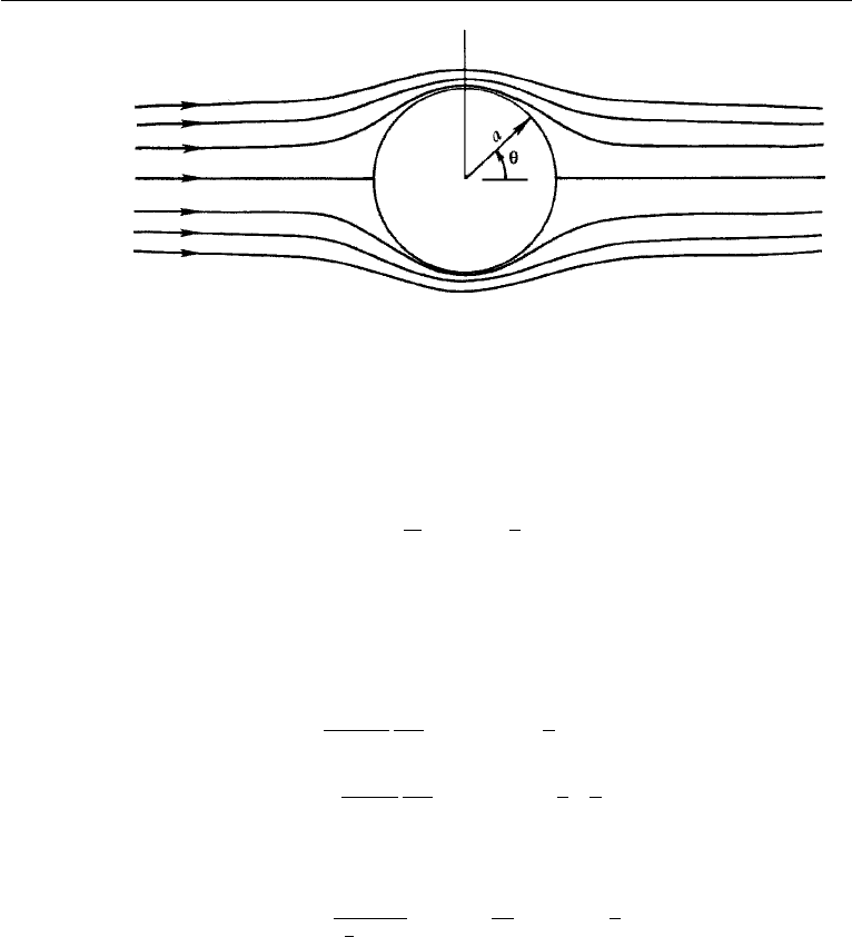
Figure 6.29 Irrotational ﬂow past a sphere.

Flow around a Sphere

Irrotational ﬂow around a sphere can be generated by the superposition of a uniform

stream and an axisymmetric doublet opposing the stream. The stream function is

ψ =−

sin

θ +

sin

θ. (6.79)

This shows that ψ = 0 for θ = 0orπ (any r), or for r = (2m/U )

1/3

(any θ ).

Thus all of the x-axis and the spherical surface of radius a = (2m/U )

1/3

form the

streamsurface ψ = 0. Streamlines of the ﬂow are shown in Figure 6.29. In terms of

the radius of the sphere, velocity components are found from equation (6.79) as

sin θ

∂ψ

∂θ

= U



1 −







cos θ,

=−

r sin θ

∂ψ

∂r

=−U



1 +







sin θ.

(6.80)

The pressure coefﬁcient on the surface is

p − p

∞

ρU

= 1 −





= 1 −

sin

θ, (6.81)

which is symmetrical, again demonstrating zero drag in steady irrotational ﬂows.

20. Flow around a Streamlined Body of Revolution

As in plane ﬂows, the motion around a closed body of revolution can be generated

by superposition of a source and a sink of equal strength on a uniform stream. The

closed surface becomes “streamlined” (that is, has a gradually tapering tail) if, for

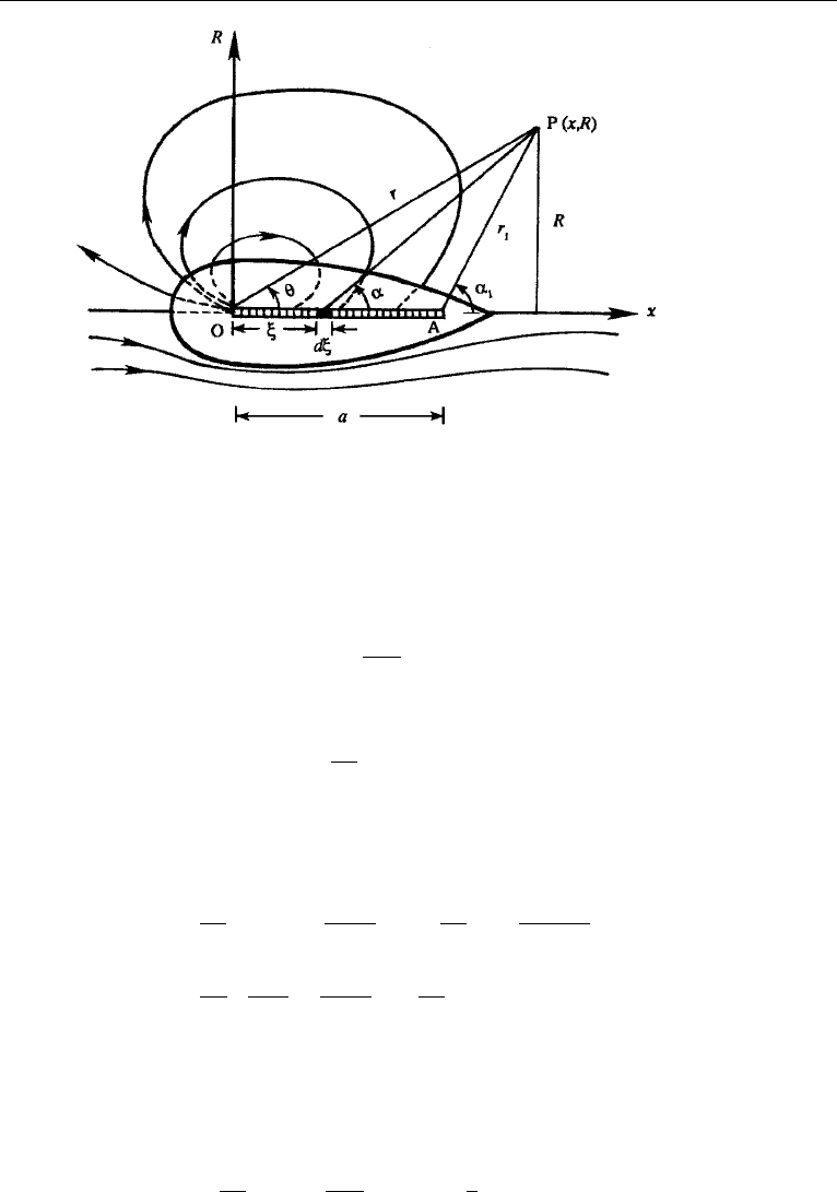
example, the sink is distributed over a ﬁnite length. Consider Figure 6.30, where there

is a point source Q(m

/s) at the origin O, and a line sink distributed on the x-axis

20. Flow around a Streamlined Body of Revolution 207

Figure 6.30 Irrotational ﬂow past a streamlined body generated by a point source at O and a distributed

line sink from O to A.

from O to A. Let the volume absorbed per unit length of the line sink be k(m

/s).

An elemental length dξ of the sink can be regarded as a point sink of strength kdξ,

for which the streamfunction at any point P is [see equation (6.77)]

dψ

sink

kdξ

4π

cos α.

The total streamfunction at P due to the entire line sink from O to A is

sink

4π



cos αdξ. (6.82)

The integral can be evaluated by noting that x − ξ = R cot α. This gives dξ =

Rdα/sin

α because x and R remain constant as we go along the sink. The stream-

function of the line sink is therefore

sink

4π



cos α

sin

dα =

4π



d(sin α)

sin

4π



sin θ

−

sin α



4π

(r − r

). (6.83)

To obtain a closed body, we must adjust the strengths so that the efﬂux from the source

is absorbed by the sink, that is, Q = ak. Then the streamfunction at any point P due

to the superposition of a point source of strength Q, a distributed line sink of strength

k = Q/a, and a uniform stream of velocity U along the x-axis, is

ψ =−

4π

cos θ +

4πa

(r − r

) +

sin

θ. (6.84)

208 Irrotational Flow

A plot of the steady streamline pattern is shown in the bottom half of Figure 6.30,

in which the top half shows instantaneous streamlines in a frame of reference at rest

with the ﬂuid at inﬁnity.

Here we have assumed that the strength of the line sink is uniform along its

length. Other interesting streamlines can be generated by assuming that the strength

k(ξ) is nonuniform.

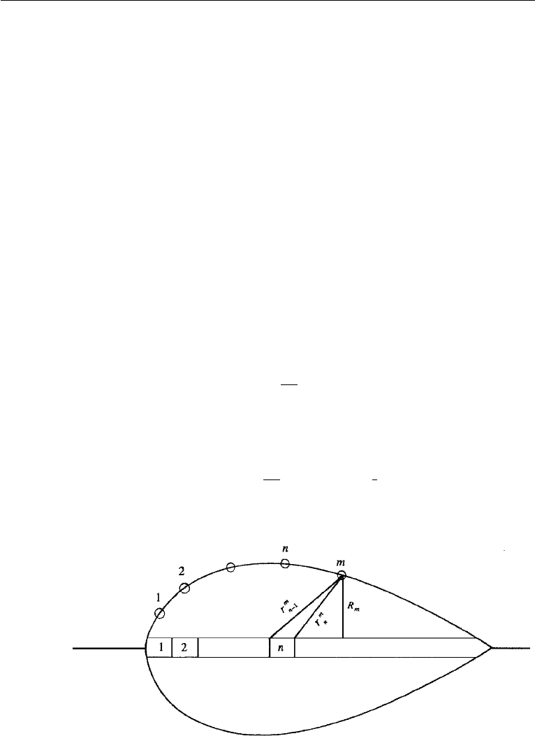
21. Flow around an Arbitrary Body of Revolution

So far, in this chapter we have been assuming certain distributions of singularities, and

determining what body shape results when the distribution is superposed on a uniform

stream. The ﬂow around a body of given shape can be simulated by superposing a

uniform stream on a series of sources and sinks of unknown strength distributed on a

line coinciding with the axis of the body. The strengths of the sources and sinks are then

so adjusted that, when combined with a given uniform ﬂow, a closed streamsurface

coincides with the given body. The calculation is done numerically using a computer.

Let the body length L be divided into N equal segments of length ξ , and let k

be the strength (m

/s) of one of these line sources, which may be positive or negative

(Figure 6.31). Then the streamfunction at any “body point” m due to the line source

n is, using equation (6.83),

=−

4π



n−1

− r



where the negative sign is introduced because equation (6.83) is for a sink. When

combined with a uniform stream, the streamfunction at m due to all N line sources is

=−



n=1

4π



n−1

− r



Figure 6.31 Flow around an arbitrary axisymmetric shape generated by superposition of a series of line

sources.

Exercise 209

Setting ψ

= 0 for all N values of m, we obtain a set of N linear algebraic equations

in N unknowns k

(n = 1, 2,...,N), which can be solved by the iteration technique

described in Section 16 or some other matrix inversion routine.

22. Concluding Remarks

The theory of potential ﬂow has reached a highly developed stage during the last

250 years because of the efforts of theoretical physicists such as Euler, Bernoulli,

D’Alembert, Lagrange, Stokes, Helmholtz, Kirchhoff, and Kelvin. The special inter-

est in the subject has resulted from the applicability of potential theory to other ﬁelds

such as heat conduction, elasticity, and electromagnetism. When applied to ﬂuid ﬂows,

however, the theory resulted in the prediction of zero drag on a body at variance with

observations. Meanwhile, the theory of viscous ﬂow was developed during the mid-

dle of the Nineteenth Century, after the Navier–Stokes equations were formulated.

The viscous solutions generally applied either to very slow ﬂows where the nonlinear

advection terms in the equations of motion were negligible, or to ﬂows in which the

advective terms were identically zero (such as the viscous ﬂow through a straight

pipe). The viscous solutions were highly rotational, and it was not clear where the

irrotational ﬂow theory was applicable and why. This was left for Prandtl to explain,

as will be shown in Chapter 10.

It is probably fair to say that the theory of irrotational ﬂow does not occupy the

center stage in ﬂuid mechanics any longer, although it did so in the past. However,

the subject is still quite useful in several ﬁelds, especially in aerodynamics. We shall

see in Chapter 10 that the pressure distribution around streamlined bodies can still be

predicted with a fair degree of accuracy from the irrotational ﬂow theory. In Chapter 15

we shall see that the lift of an airfoil is due to the development of circulation around

it, and the magnitude of the lift agrees with the Kutta–Zhukhovsky lift theorem. The

technique of conformal mapping will also be essential in our study of ﬂow around

airfoil shapes.

Exercises

1. In Section 7, the doublet potential

w = µ/z,

was derived by combining a source and a sink on the x-axis. Show that the same

potential can also be obtained by superposing a clockwise vortex of circulation −

on the y-axis at y = ε, and a counterclockwise vortex of circulation  at y =−ε,

and letting ε → 0.

2. By integrating pressure, show that the drag on a plane half-body (Section 8)

is zero.

3. Graphically generate the streamline pattern for a plane half-body in the fol-

lowing manner. Take a source of strength m = 200 m

/s and a uniform stream U =

10 m/s. Draw radial streamlines from the source at equal intervals of θ = π/10,

210 Irrotational Flow

with the corresponding streamfunction interval

ψ

source

2π

θ = 10 m

/s.

Now draw streamlines of the uniform ﬂow with the same interval, that is,

ψ

stream

= Uy= 10 m

/s.

This requires y = 1 m, which you can plot assuming a linear scale of 1 cm = 1m.

Now connect points of equal ψ = ψ

source

+ψ

stream

. (Most students enjoy doing this

exercise!)

4. Take a plane source of strength m at point (−a, 0), a plane sink of equal

strength at (a, 0), and superpose a uniform stream U directed along the x-axis. Show

that there are two stagnation points located on the x-axis at points

±a



πaU

+ 1



1/2

Show that the streamline passing through the stagnation points is given by ψ = 0.

Verify that the line ψ = 0 represents a closed oval-shaped body, whose maximum

width h is given by the solution of the equation

h = a cot



πUh



The body generated by the superposition of a uniform stream and a source–sink pair is

called a Rankine body. It becomes a circular cylinder as the source–sink pair approach

each other.

5. A two-dimensional potential vortex with clockwise circulation  is located at

point (0,a) above a ﬂat plate. The plate coincides with the x-axis. A uniform stream

U directed along the x-axis ﬂows over the vortex. Sketch the ﬂow pattern and show

that it represents the ﬂow over an oval-shaped body. [Hint: Introduce the image vortex

and locate the two stagnation points on the x-axis.]

If the pressure at x =±∞is p

∞

, and that below the plate is also p

∞

, then show

that the pressure at any point on the plate is given by

∞

− p =

ρ

2π

+ a

)

−

ρUa

π(x

+ a

)

Show that the total upward force on the plate is

F =

ρ

4πa

− ρU.

6. Consider a point source of strength Q(m

/s). Argue that the velocity com-

ponents in spherical coordinates are u

= 0 and u

= Q/4πr

and that the velocity

Exercises 211

potential and streamfunction must be of the form φ = φ(r)and ψ = ψ(θ). Integrating

the velocity, show that φ =−Q/4πr and ψ =−Q cos θ/4π.

7. Consider a point doublet obtained as the limiting combination of a point

source and a point sink as the separation goes to zero. (See Section 7 for its two

dimensional counterpart.) Show that the velocity potential and streamfunction in

spherical coordinates are φ = m cos θ/r

and ψ =−m sin

θ/r, where m is the

limiting value of Qδs/4π , with Q as the source strength and δs as the separation.

8. A solid hemisphere of radius a is lying on a ﬂat plate. A uniform stream

U is ﬂowing over it. Assuming irrotational ﬂow, show that the density of the material

must be

 ρ



1 +



to keep it on the plate.

9. Consider the plane ﬂow around a circular cylinder. Use the Blasius theorem

equation (6.45) to show that the drag is zero and the lift is L = ρU. (In Section 10,

we derived these results by integrating the pressure.)

10. There is a point source of strength Q(m

/s) at the origin, and a uniform

line sink of strength k = Q/a extending from x = 0tox = a. The two are combined

with a uniform stream U parallel to the x-axis. Show that the combination represents

the ﬂow past a closed surface of revolution of airship shape, whose total length is the

difference of the roots of



± 1



4πUa

11. Using a computer, determine the surface contour of an axisymmetric

half-body formed by a line source of strength k(m

/s) distributed uniformly along

the x-axis from x = 0tox = a and a uniform stream. Note that the nose is more

pointed than that formed by the combination of a point source and a uniform stream.

By a mass balance (see Section 8), show that the far downstream asymptotic radius

of the half-body is r =

√

ak/πU .

12. For the ﬂow described by equation (6.30) and sketched in Figure 6.8, show

for µ>0 that u<0 for y<xand u>0 for y>x. Also, show that v<0 in the

ﬁrst quadrant and v>0 in the second quadrant.

13. A hurricane is blowing over a long “Quonset hut,” that is, a long half-circular

cylindrical cross-section building, 6 m in diameter. If the velocity far upstream is

∞

= 40 m/s and p

∞

= 1.003 × 10

N/m, ρ

∞

= 1.23 kg/m

, ﬁnd the force per

unit depth on the building, assuming the pressure inside is p

∞

14. In a two-dimensional constant density potential ﬂow, a source of strength m

is located a meters above an inﬁnite plane. Find the velocity on the plane, the pressure

on the plane, and the reaction force on the plane.