Cohen I.M., Kundu P.K. Fluid Mechanics

Подождите немного. Документ загружается.

192 Irrotational Flow

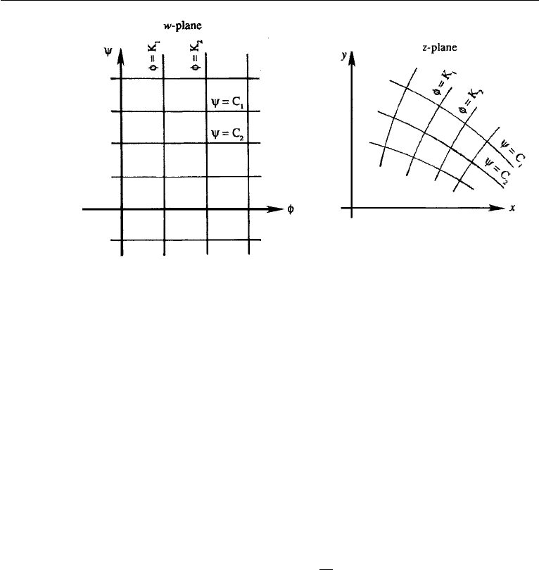
Figure 6.20 Flow patterns in the w-plane and the z-plane.

A simple example of conformal mapping is given immediately below as a special case

of the ﬂow discussed in Section 4 above. Consider the transformation, w = φ + iψ =

= x

− y

+ 2ixy. Streamlines are ψ = const = 2xy, rectangular hyperbolae.

See one quadrant of the ﬂow depicted in Fig. 6.5. Uniform ﬂow in the w-plane has

been mapped onto ﬂow in a right hand corner in the z-plane by this transformation.

A more involved example is shown in the next section. Additional applications are

discussed in Chapter 15.

14. Flow around an Elliptic Cylinder with Circulation

We shall brieﬂy illustrate the method of conformal mapping by considering a trans-

formation that has important applications in airfoil theory. Consider the following

transformation:

z = ζ +

, (6.53)

relating z and ζ planes. We shall now show that a circle of radius b centered at the

origin of the ζ -plane transforms into a straight line on the real axis of the z-plane. To

prove this, consider a point ζ = b exp (iθ) on the circle (Figure 6.21), for which the

corresponding point in the z-plane is

z = be

iθ

+ be

−iθ

= 2b cos θ.

As θ varies from 0 to π , z goes along the x-axis from 2b to −2b.Asθ varies from π

to 2π, z goes from −2b to 2b. The circle of radius b in the ζ -plane is thus transformed

into a straight line of length 4b in the z-plane. It is clear that the region outside

the circle in ζ -plane is mapped into the entire z-plane. It can be shown that the

region inside the circle is also transformed into the entire z-plane. This, however, is

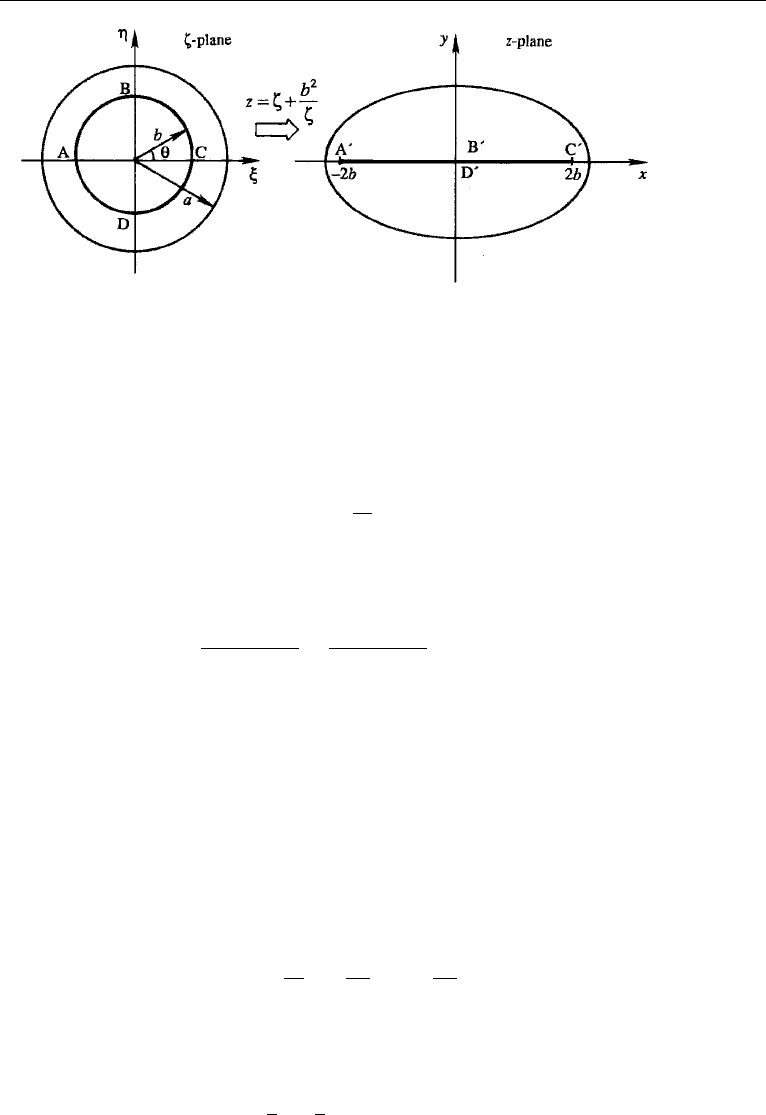
14. Flow around an Elliptic Cylinder with Circulation 193

Figure 6.21 Transformation of a circle into an ellipse by means of the Zhukhovsky transformation

z = ζ + b

/ζ .

of no concern to us because we shall not consider the interior of the circle in the

ζ -plane.

Now consider a circle of radius a>b in the ζ -plane (Figure 6.21). Points

ζ = a exp (iθ) on this circle are transformed to

z = ae

iθ

−iθ

, (6.54)

which traces out an ellipse for various values of θ . This becomes clear by elimination

of θ in equation (6.54), giving

(a + b

/a)

(a − b

/a)

= 1. (6.55)

For various values of a>b, equation (6.55) represents a family of ellipses in the

z-plane, with foci at x =±2b.

The ﬂow around one of these ellipses (in the z-plane) can be determined by

ﬁrst ﬁnding the ﬂow around a circle of radius a in the ζ -plane, and then using

the transformation equation (6.53) to go to the z-plane. To be speciﬁc, suppose the

desired ﬂow in the z-plane is that of ﬂow around an elliptic cylinder with clockwise

circulation , which is placed in a stream moving at U. The corresponding ﬂow in

the ζ -plane is that of ﬂow with the same circulation around a circular cylinder of

radius a placed in a stream of the same strength U for which the complex potential

is (see equation (6.37))

w = U



ζ +



i

2π

ln ζ −

i

2π

ln a. (6.56)

The complex potential w(z) in the z-plane can be found by substituting the inverse

of equation (6.53), namely,

ζ =

z +

− 4b

)

1/2

, (6.57)

194 Irrotational Flow

into equation (6.56). (Note that the negative root, which falls inside the cylinder, has

been excluded from equation (6.57).) Instead of ﬁnding the complex velocity in the

z-plane by directly differentiating w(z), it is easier to ﬁnd it as

u − iv =

dζ

The resulting ﬂow around an elliptic cylinder with circulation is qualitatively quite

similar to that around a circular cylinder as shown in Figure 6.14.

15. Uniqueness of Irrotational Flows

In Section 10 we saw that plane irrotational ﬂow over a cylindrical object is nonunique.

In particular, ﬂows with any amount of circulation satisfy the same boundary

conditions on the body and at inﬁnity. With such an example in mind, we are ready

to make certain general statements concerning solutions of the Laplace equation. We

shall see that the topology of the region of ﬂow has a great inﬂuence on the uniqueness

of the solution.

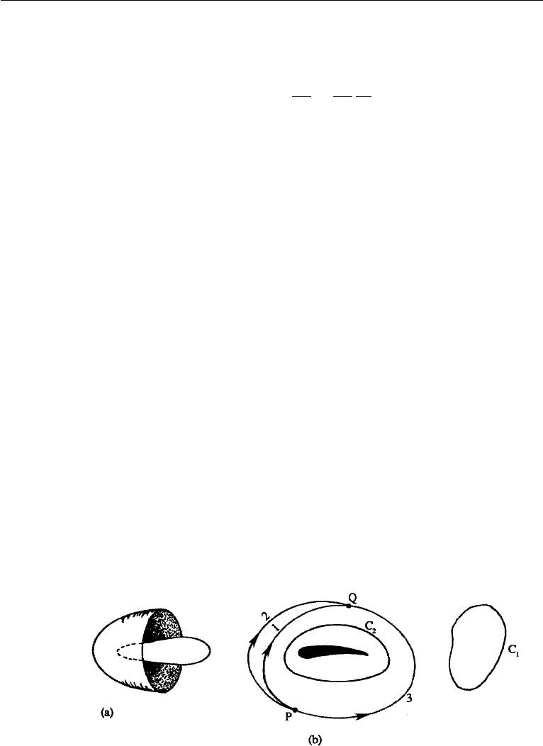
Before we can make these statements, we need to deﬁne certain terms. A reducible

circuit is any closed curve (lying wholly in the ﬂow ﬁeld) that can be reduced to a

point by continuous deformation without ever cutting through the boundaries of the

ﬂow ﬁeld. We say that a region is singly connected if every closed circuit in the region

is reducible. For example, the region of ﬂow around a ﬁnite body of revolution is

reducible (Figure 6.22a). In contrast, the ﬂow ﬁeld over a cylindrical object of inﬁnite

length is multiply connected because certain circuits (such as C

in Figure 6.22b) are

reducible while others (such as C

) are not reducible.

To see why solutions are nonunique in a multiply connected region, consider the

two circuits C

and C

in Figure 6.22b. The vorticity everywhere within C

is zero,

thus Stokes’ theorem requires that the circulation around it must vanish. In contrast,

the circulation around C

can have any strength . That is,



•

dx = , (6.58)

Figure 6.22 Singly connected and multiply connected regions: (a) singly connected; (b) multiply

connected.

16. Numerical Solution of Plane Irrotational Flow 195

where the loop around the integral sign has been introduced to emphasize that the

circuit C

is closed. As the right-hand side of equation (6.58) is nonzero, it follows

that u

•

dx is not a “perfect differential,” which means that the line integral between

any two points depends on the path followed (u

•

dx is called a perfect differential

if it can be expressed as the differential of a function, say as u

•

dx = df . In that

case the line integral around a closed circuit must vanish). In Figure 6.22b, the line

integrals between P and Q are the same for paths 1 and 2, but not the same for paths 1

and 3. The solution is therefore nonunique, as was physically evident from the whole

family of irrotational ﬂows shown in Figure 6.14.

In singly connected regions, circulation around every circuit is zero, and the solu-

tion of ∇

φ = 0 is unique when values of φ are speciﬁed at the boundaries (the

Dirichlet problem). When normal derivatives of φ are speciﬁed at the boundary (the

Neumann problem), as in the ﬂuid ﬂow problems studied here, the solution is unique

within an arbitrary additive constant. Because the arbitrary constant is of no conse-

quence, we shall say that the solution of the irrotational ﬂow in a singly connected

region is unique. (Note also that the solution depends only on the instantaneous

boundary conditions; the differential equation ∇

φ = 0 is independent of t.)

Summary: Irrotational ﬂow around a plane two-dimensional object is non-

unique because it allows an arbitrary amount of circulation. Irrotational ﬂow around

a ﬁnite three-dimensional object is unique because there is no circulation.

In Sections 4 and 5 of Chapter 5 we learned that vorticity is solenoidal (∇·ω = 0),

or that vortex lines cannot begin or end anywhere in the ﬂuid. Here we have learned

that a circulation in a two dimensional ﬂow results in a force normal to an oncoming

stream. This is used to simulate lifting ﬂow over a wing by the following artiﬁce,

discussed in more detail in our chapter on Aerodynamics. Since Stokes’ theorem tells

us that the circulation about a closed contour is equal to the ﬂux of vorticity through

any surface bounded by that contour, the circulation about a thin airfoil section is

simulated by a continuous row of vortices (a vortex sheet) along the centerline of

a wing cross-section (the mean camber line of an airfoil). For a (real) ﬁnite wing,

these vortices must bend downstream to form trailing vortices and terminate in starting

vortices (far downstream), always forming closed loops. Although the wing may be

a ﬁnite three dimensional shape, the contour cannot cut any of the vortex lines without

changing the circulation about the contour. Generally, the circulation about a wing

does vary in the spanwise direction, being a maximum at the root or centerline and

tending to zero at the wingtips.

Additional boundary conditions that the mean camber line be a streamline and

that a real trailing edge be a stagnation point serve to render the circulation distribution

unique.

16. Numerical Solution of Plane Irrotational Flow

Exact solutions can be obtained only for ﬂows with simple geometries, and approxi-

mate methods of solution become necessary for practical ﬂow problems. One of these

approximate methods is that of building up a ﬂow by superposing a distribution of

sources and sinks; this method is illustrated in Section 21 for axisymmetric ﬂows.

196 Irrotational Flow

Another method is to apply perturbation techniques by assuming that the body is thin.

A third method is to solve the Laplace equation numerically. In this section we shall

illustrate the numerical method in its simplest form. No attempt is made here to use

the most efﬁcient method. It is hoped that the reader will have an opportunity to learn

numerical methods that are becoming increasingly important in the applied sciences

in a separate study. See Chapter 11 for introductory material on several important

techniques of computational ﬂuid dynamics.

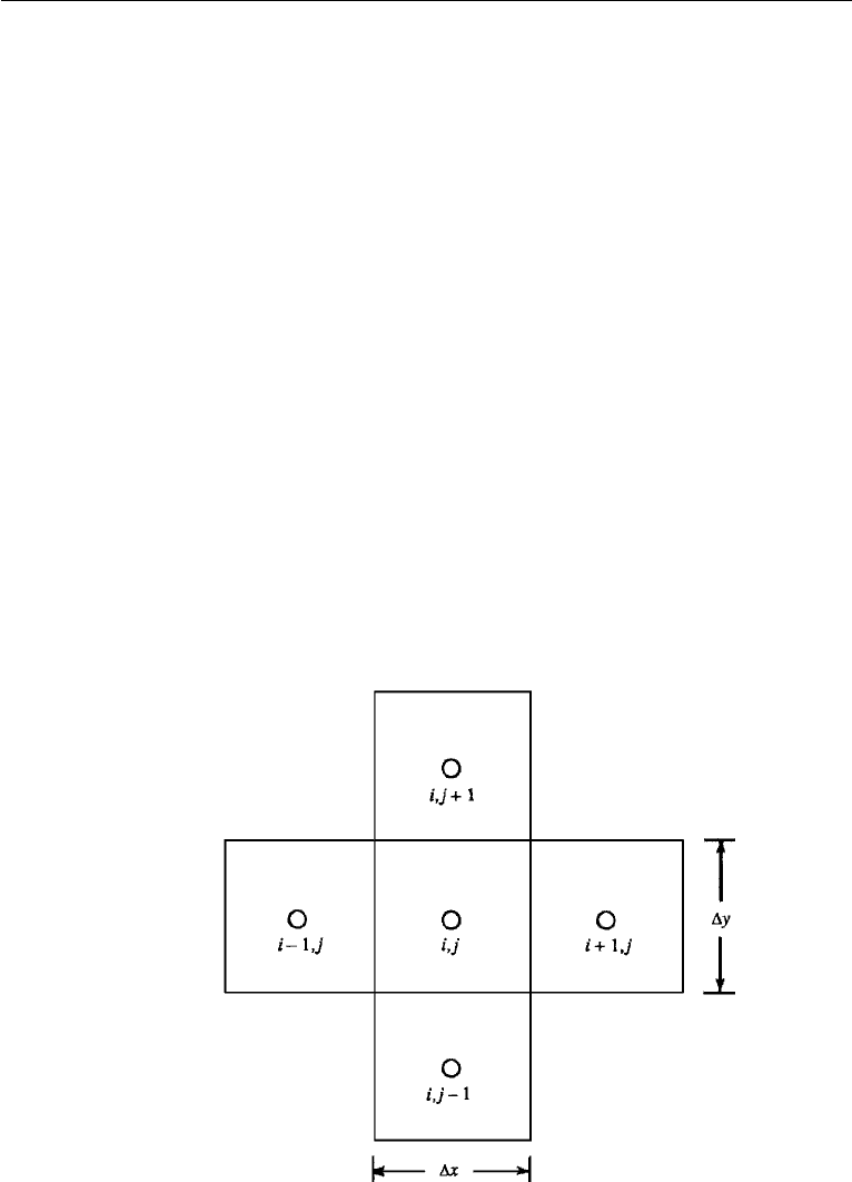
Finite Difference Form of the Laplace Equation

In ﬁnite difference techniques we divide the ﬂow ﬁeld into a system of grid points,

and approximate the derivatives by taking differences between values at adjacent grid

points. Let the coordinates of a point be represented by

x = ix (i = 1, 2,...,),

y = jy (j = 1, 2,...,).

Here, x and y are the dimensions of a grid box, and the integers i and j are the

indices associated with a grid point (Figure 6.23). The value of a variable ψ(x, y)

can be represented as

ψ(x, y) = ψ(i x,j y) ≡ ψ

i,j

Figure 6.23 Adjacent grid boxes in a numerical calculation.

16. Numerical Solution of Plane Irrotational Flow 197

where ψ

i,j

is the value of ψ at the grid point (i, j). In ﬁnite difference form, the ﬁrst

derivatives of ψ are approximated as



∂ψ

∂x



i,j



x



− ψ

i−





∂ψ

∂y



i,j



y



i,j+

− ψ

i,j−



The quantities on the right-hand side (such as ψ

i+1/2,j

) are half-way between the

grid points and therefore undeﬁned. However, this would not be a difﬁculty in the

present problem because the Laplace equation does not involve ﬁrst derivatives. Both

derivatives are written as ﬁrst-order centered differences.

The ﬁnite difference form of ∂

ψ/∂x



∂

∂x



i,j



x





∂ψ

∂x



−



∂ψ

∂x



i−





x



x

(ψ

i+1,j

− ψ

i,j

) −

x

(ψ

i,j

− ψ

i−1,j

)



x

[ψ

i+1,j

− 2ψ

i,j

+ ψ

i−1,j

]. (6.59)

Similarly,



∂

∂y



i,j



y

[ψ

i,j+1

− 2ψ

i,j

+ ψ

i,j−1

] (6.60)

Using equations (6.59) and (6.60), the Laplace equation for the streamfunction in a

plane two-dimensional ﬂow

∂

∂x

∂

∂y

= 0,

has a ﬁnite difference representation

x

[ψ

i+1,j

− 2ψ

i,j

+ ψ

i−1,j

y

[ψ

i,j+1

− 2ψ

i,j

+ ψ

i,j−1

]=0.

Taking x = y, for simplicity, this reduces to

i,j

[ψ

i−1,j

+ ψ

i+1,j

+ ψ

i,j−1

+ ψ

i,j+1

], (6.61)

which shows that ψ satisﬁes the Laplace equation if its value at a grid point equals

the average of the values at the four surrounding points.

198 Irrotational Flow

Simple Iteration Technique

We shall now illustrate a simple method of solution of equation (6.61) when the values

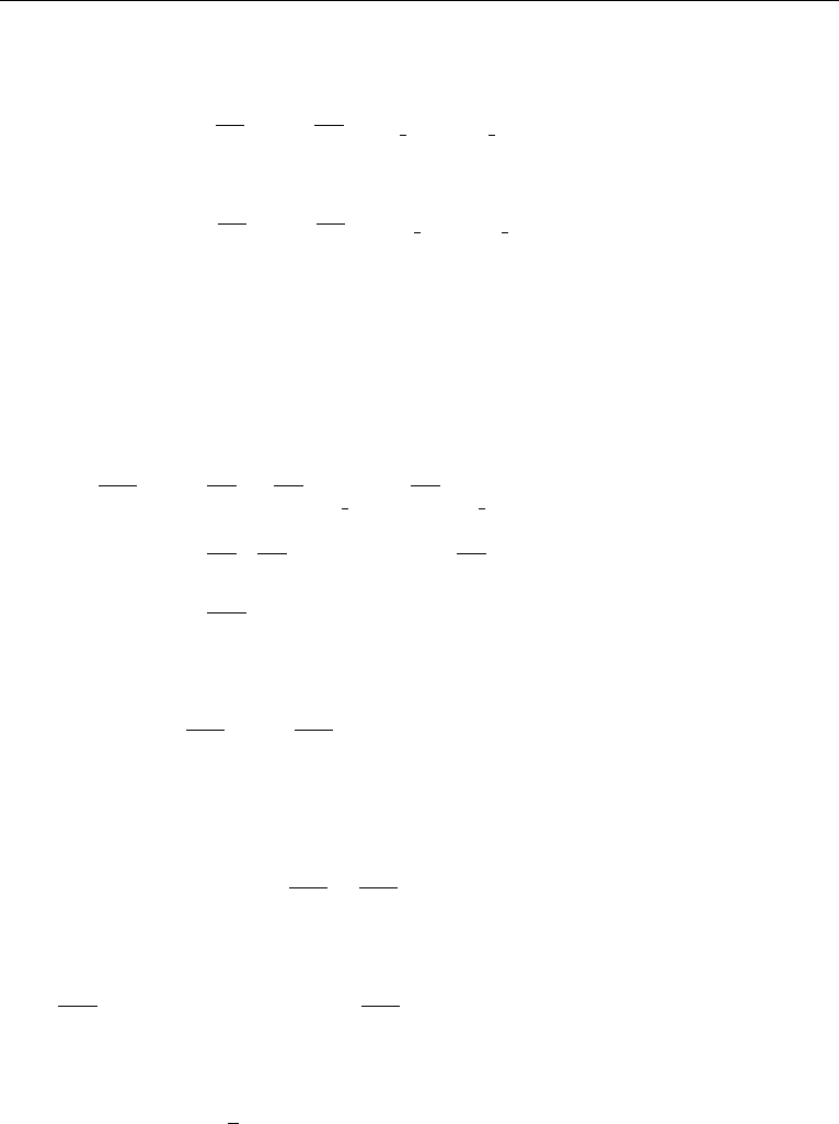
of ψ are given in a simple geometry. Assume the rectangular region of Figure 6.24,

in which the ﬂow ﬁeld is divided into 16 grid points. Of these, the values of ψ are

known at the 12 boundary points indicated by open circles. The values of ψ at the

four interior points indicated by solid circles are unknown. For these interior points,

the use of equation (6.61) gives

2,2



1,2

+ ψ

3,2

+ ψ

2,1

+ ψ

2,3



3,2



2,2

+ ψ

4,2

+ ψ

3,1

+ ψ

3,3



2,3



1,3

+ ψ

3,3

+ ψ

2,2

+ ψ

2,4



3,3



2,3

+ ψ

4,3

+ ψ

3,2

+ ψ

3,4



(6.62)

Figure 6.24 Network of grid points in a rectangular region. Boundary points with known values are

indicated by open circles. The four interior points with unknown values are indicated by solid circles.

16. Numerical Solution of Plane Irrotational Flow 199

In the preceding equations, the known boundary values have been indicated by a

superscript “B.” Equation set (6.62) represents four linear algebraic equations in four

unknowns and is therefore solvable.

In practice, however, the ﬂow ﬁeld is likely to have a large number of grid points,

and the solution of such a large number of simultaneous algebraic equations can only

be performed using a computer. One of the simplest techniques of solving such a

set is the iteration method. In this a solution is initially assumed and then gradually

improved and updated until equation (6.61) is satisﬁed at every point. Suppose the

values of ψ at the four unknown points of Figure 6.24 are initially taken as zero.

Using equation (6.62), the ﬁrst estimate of ψ

2,2

can be computed as

2,2



1,2

+ 0 + ψ

2,1

+ 0



The old zero value for ψ

2,2

is now replaced by the preceding value. The ﬁrst estimate

for the next grid point is then obtained as

3,2



2,2

+ ψ

4,2

+ ψ

3,1

+ 0



where the updated value of ψ

2,2

has been used on the right-hand side. In this manner,

we can sweep over the entire region in a systematic manner, always using the latest

available value at the point. Once the ﬁrst estimate at every point has been obtained,

we can sweep over the entire region once again in a similar manner. The process is

continued until the values of ψ

i,j

do not change appreciably between two successive

sweeps. The iteration process has now “converged.”

The foregoing scheme is particularly suitable for implementation using a com-

puter, whereby it is easy to replace old values at a point as soon as a new value

is available. In practice, a more efﬁcient technique, for example, the successive

over-relaxation method, will be used in a large calculation. The purpose here is not to

describe the most efﬁcient technique, but the one which is simplest to illustrate. The

following example should make the method clear.

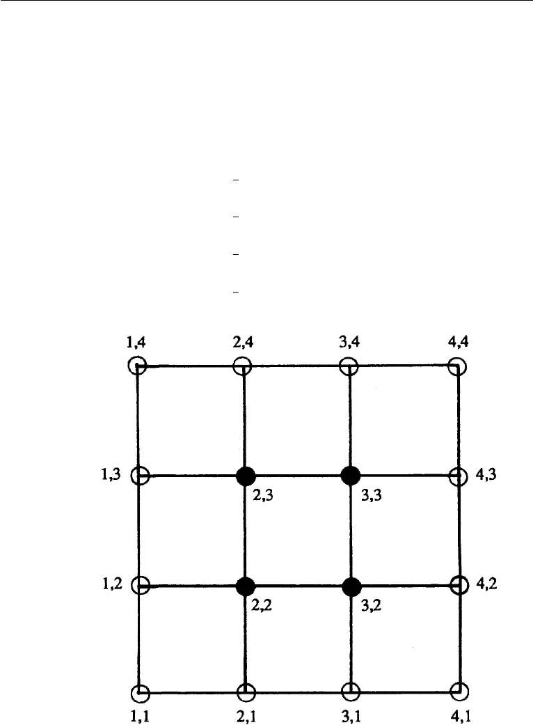
Example 6.1. Figure 6.25 shows a contraction in a channel through which the ﬂow

rate per unit depth is 5 m

/s. The velocity is uniform and parallel across the inlet and

outlet sections. Find the ﬂow ﬁeld.

Solution: Although the region of ﬂow is plane two-dimensional, it is clearly

singly connected. This is because the ﬂow ﬁeld interior to a boundary is desired, so

that every ﬂuid circuit can be reduced to a point. The problem therefore has a unique

solution, which we shall determine numerically.

We know that the difference in ψ values is equal to the ﬂow rate between two

streamlines. If we take ψ = 0 at the bottom wall, then we must have ψ = 5m

/satthe

top wall. We divide the ﬁeld into a system of grid points shown, with x = y = 1m.

Because ψ/y (= u) is given to be uniform across the inlet and the outlet, we must

have ψ = 1m

/s at the inlet and ψ = 5/3 = 1.67 m

/s at the outlet. The

resulting values of ψ at the boundary points are indicated in Figure 6.25.

200 Irrotational Flow

Figure 6.25 Grid pattern for irrotational ﬂow through a contraction (Example 16). The boundary values

of ψ are indicated on the outside. The values of i,j for some grid points are indicated on the inside.

The FORTRAN code for solving the problem is as follows:

DIMENSION S(10, 6)

DO 10 I=1,6

10 S(I, 1) = 0.

DO 20 J=2,3

20 S(6, J) = 0.

DO 30 I=7,10

30 S(I, 3) = 0.

DO 40 I=1,10

40 S(I, 6) = 5.











Set ψ = 0 on top and bottom walls

DO 50 J=2,6

50 S(1, J) = J - 1.



Set ψ at inlet

DO 60 J=4,6

60 S(10, J) = (J - 3) * (5. / 3.)



Set ψ at outlet

DO 100 N = 1, 20

DO 70 I=2,5

DO 70 J=2,5

70 S(I, J) = (S(I,J+1)+S(I, J-1) + S(I + 1, J) + S(I - 1, J)) / 4.

DO 80 I=6,9

DO 80 J=4,5

80 S(I, J) = (S(I,J+1)+S(I,J-1)+S(I+1,J)+S(I-1,J))/4.

100 CONTINUE

PRINT 1, ((S(I, J),I=1,10),J=1,6)

1 FORMAT (' ', 10 E 12.4)

END

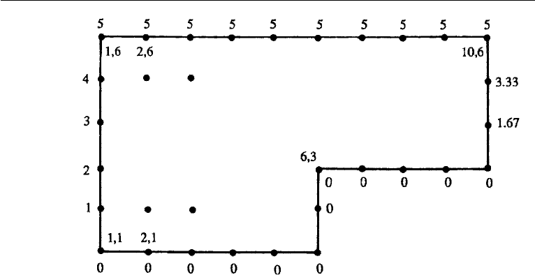
17. Axisymmetric Irrotational Flow 201

Figure 6.26 Numerical solution of Example 6.1.

Here, S denotes the stream function ψ. The code ﬁrst sets the boundary values.

The iteration is performed in the N loop. In practice, iterations will not be performed

arbitrarily 20 times. Instead the convergence of the iteration process will be checked,

and the process is continued until some reasonable criterion (such as less than 1%

change at every point) is met. These improvements are easy to implement, and the

code is left in its simplest form.

The values of ψ at the grid points after 50 iterations, and the corresponding

streamlines, are shown in Figure 6.26.

It is a usual practice to iterate until successive iterates change only by a prescribed

small amount. The solution is then said to have “converged.” However, a caution is

in order. To be sure a solution has been obtained, all of the terms in the equation

must be calculated and the satisfaction of the equation by the “solution” must be

veriﬁed.

17. Axisymmetric Irrotational Flow

Several examples of irrotational ﬂow around plane two-dimensional bodies were

given in the preceding sections. We used Cartesian (x,y) and plane polar (r, θ )

coordinates, and found that the problem involved the solution of the Laplace equa-

tion in φ or ψ with speciﬁed boundary conditions. We found that a very power-

ful tool in the analysis was the method of complex variables, including conformal

transformation.

Two streamfunctions are required to describe a fully three-dimensional

ﬂow (Chapter 4, Section 4), although a velocity potential (which satisﬁes the

three-dimensional version of ∇

φ = 0) can be deﬁned if the ﬂow is irrotational.