Blum W., Riegler W., Rolandi L. Particle Detection with Drift Chambers

Подождите немного. Документ загружается.

Chapter 10

Particle Identiﬁcation by Measurement

of Ionization

Among the track parameters, the ionization plays a special role because it is a

function of the particle velocity, which can therefore be indirectly determined

through a measurement of the amount of ionization along a track. For relativistic

particles this dependence is not very strong, and therefore the amount of ionization

must be measured accurately in order to be useful. The ionization has a very broad

distribution, and a track has to be measured on many segments (several tens to a few

hundred) in order to reach the accuracy required. Fortunately only relative values of

the ionization need to be known between tracks of different velocities.

Whereas in Chap. 1 we dealt with the ionization phenomenon in general terms,

the present chapter is devoted to a discussion of those aspects of ionization that

are important for particle identiﬁcation. After an explanation of the principle we

elaborate on the factors that determine the shape of the ionization curve, and the

achievable accuracy. Calculated and measured particle separation powers are dis-

cussed next. One section is devoted to cluster counting. Finally, the problems

encountered in practical devices are reviewed.

10.1 Principles

In a magnetic spectrometer one measures the particle momentum through the curva-

ture of its track in the magnetic ﬁeld. If a measurement of ionization is performed on

this track, there is the possibility of determining the particle mass, thus identifying

the particle. The relation between momentum p and velocity v involves the mass m:

v = c

p/E = c

√

+ m

), (10.1)

where c is the velocity of light.

Any quantiﬁcation of ionization involves the peculiar statistics of the ionization

process. Let us recapitulate from Chap. 1 that the distribution function of the number

of electrons produced on a given track length has such a tail towards large numbers

that neither a proper mean nor a proper variance exists for the number of electrons.

W. Blum et al., Particle Detection with Drift Chambers, 331

doi: 10.1007/978-3-540-76684-1

10,

 Springer-Verlag Berlin Heidelberg 2008

332 10 Particle Identiﬁcation by Measurement of Ionization

In order to characterize the distribution one may quote its most probable value and

its width at half-maximum. The most probable number of electrons may be taken to

represent the ‘strength’ of the ionization. It is not proportional to the length of the

track segment. (We have seen in Figs. 1.10 and 1.11 how the most probable value of

the ionization per unit length goes up with the gas sample length.) From a number of

pulse-height measurements on one track one derives some measure I of the strength

of the ionization; details are given in Sect. 10.3. Since I depends on the velocity of

the particle and is proportional to the square of the charge Ze of the particle, we

write

I = Z

g,m

(v). (10.2)

g,m

(v) depends, ﬁrstly, on the nature of the gas mixture and its density (index g).

But it depends also on the length and number of samples and on the exact way in

which the ionization of the track is calculated from the ionization of the different

samples (index m); in addition, there is the small dependence of the relativistic rise

on the sample size. If we divide F

g,m

(v) by its minimal value (at v

min

), we obtain a

normalized curve

(norm)

g,m

(v)=F

g,m

(v)/F

g,m

min

). (10.3)

It turns out that this curve is approximately independent of the exact manner of the

ionization measurement:

(norm)

g,m

(v) ≈ F

(v). (10.4)

(Some qualiﬁcations are mentioned in the end of Sect. 10.8.1) Most analyses of

the ionization loss have been done with this approximation, i.e. one neglects any

variation of the relativistic rise on the sample size and works with one universal

normalized curve.

Figure 1.19 contained theoretical values for the most probable ionization in

argon, as well as experimental values of the truncated mean in argon–methane

mixtures. The abscissa is the logarithm of

βγ

(

= v/c,

= 1/(1 −

)), and the

vertical scale is normalized to the value in the minimum.

One cannot resolve (10.1), (10.2) and (10.4) into a form m = m(I, p) because

(v) is not monotonic. Therefore we discuss particle identiﬁcation by plotting

(v) for various known charged particles as a function of p. Using the argon curve

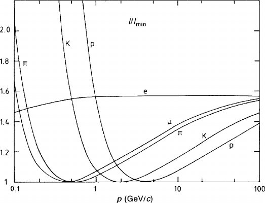
of Fig. 1.19 we obtain the family of curves shown in Fig. 10.1. We see ﬁve curves of

identical shape, for electrons, muons, pions, kaons, and protons; they are displaced

with respect to each other on the logarithmic scale by the logarithms of the particle

mass ratios.

The simultaneous measurement of the momentum and the ionization of a particle

results in a point in the diagram of Fig. 10.1. Complete particle identiﬁcation takes

place if, inside the measurement errors, this point can be associated with only one

curve. In practice the measurement errors of the ionization are very often so large

that several particles could have caused the measured ionization; if this is the case it

may be possible to exclude one or more particles.

For good particle identiﬁcation the measurement accuracy

I is obviously as

essential as the vertical distance between the curves in Fig. 10.1. It is therefore our

ﬁrst task to review the gas conditions responsible for the shape of the curve and

10.1 Principles 333

Fig. 10.1 Most probable values of the ionization (normalized to the minimum value) in argon at

ordinary density as function of the momenta of the known stable charged particles

in particular for the amount of the relativistic rise. Then we have to understand the

circumstances that have an inﬂuence on

I, and which value of

I can be reached

in a given apparatus. The ratio of the accuracy over the relativistic rise characterizes

the particle separation power.

But before going into these details let us make an estimate of what we can expect

from this method of particle identiﬁcation. Imagine some drift chamber with a rel-

ative accuracy of

I/I = 12% FWHM (5% r.m.s.). If we assume that a respectable

degree of identiﬁcation is already achievable on a curve that is only twice this r.m.s.

value away from any other one, if we remove the muon curve (because it is hope-

lessly close to the pion curve and because muons can be well identiﬁed with other

methods), and if, ﬁnally, we assume that the error of the momentum measurement is

negligible, then we can redraw those branches of the curves in Fig. 10.1 that would

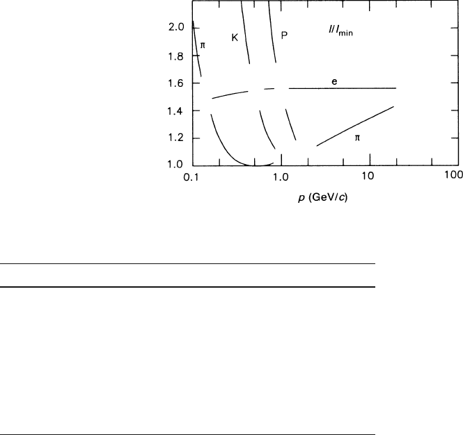
allow a respectable degree of particle identiﬁcation in argon. The result is seen in

Fig. 10.2.

Under the assumed circumstances, these particles could be identiﬁed in the

ranges shown in Table 10.1. It is characteristic of the complicated shape of the ion-

ization curve that there are certain bands of overlap in which unique identiﬁcation is

impossible. A useful separation between kaons and protons at high momenta would

require the measurement accuracy for the ionization to be

I/I = 8.5% FWHM

or better (in argon at normal density). Such values have actually been attained by

specialized particle identiﬁers, see Sect. 10.8.

After having described the principle of particle identiﬁcation based on the

amount of ionization along a given length of track we should also mention the pos-

sibility based on the frequency of ionization along the track. If we were to count the

334 10 Particle Identiﬁcation by Measurement of Ionization

Fig. 10.2 Thesameas

Fig. 10.1 with all lines left out

that either belong to a muon

or that have a neighbouring

line closer than 10% in

ionization (corresponding to a

separation of 2 standard

deviations when the r.m.s.

accuracy is 5%)

Table 10.1 Momentum ranges above 0.1 GeV/c for a 2

identiﬁcation of particles in argon

(normal density), for two measuring accuracies of the ionization (μ’s removed)

Particle Momentum ranges (GeV/c)

I/I = 5% r.m.s.

e 0.17–0.4 0.6–0.8 1.3–19

(0.1)–0.12 0.16–0.8 2.7–19

K (0.1)–0.4 0.6–0.8

p (0.1)–0.8 1.1–1.5

I/I = 3.5% r.m.s.

e 0.16–0.5 0.6–0.9 1.1–30

(0.1)–0.13 0.16–0.9 2.2–30

K (0.1)–0.5 0.6–0.9 6–46

p (0.1)–0.9 1.1–1.5 6–46

number of ionization clusters rather than the amount of ionization on some track

length, there would be a proﬁt in the statistical accuracy. A brief description of this

interesting method is given in Sect. 10.6.

Much easier than the identiﬁcation of the known particles would be the recog-

nition of a stable quark with charge e/3or2e/3, because it would create only 1/9

or 4/9 of the normal ionization density. Quarks aside, one recognizes that relatively

small differences in

I/I may be decisive for particle identiﬁcation. Therefore we

must study in some detail how the shape of the ionization curve and the achievable

accuracy depend on the parameters of the drift chamber.

10.2 Shape of the Ionization Curve

We recall from Chap. 1 that the curve reaches its minimum near

βγ

= 4. The shape

of a curve that has been normalized to this minimum is characterized by the height

of the plateau (‘amount of relativistic rise’, R, above the minimum) and by the value

10.2 Shape of the Ionization Curve 335

Table 10.2 Performance of different gases according to calculations with the PAI model [ALL 82].

A track of 1 m length, sampled in 66 layers of 1.5 cm is assumed. See text for explanation

Gas R (% of min. value) W

S at 4 GeV/cSat 20 GeV/c

Peak lower upper (% FWHM) e-

ππ

–K K–p e–

ππ

–K K–p

He 58 86 45 15 1.5 0.9 0.3 0.3 0.9 0.5

Ne 57 72 57 13 1.8 1.1 0.4 0.6 1.1 0.6

Ar 57 66 49 12 1.6 1.1 0.4 0.6 0.9 0.6

Kr 63 65 61 11 2.2 1.3 0.5 0.9 1.1 0.7

Xe 67 76 64 13 2.2 1.2 0.4 1.0 1.0 0.6

56 59 48 11 1.8 1.3 0.4 0.7 1.0 0.7

54 54 47 9 2.0 1.5 0.5 0.7 1.1 0.8

48 52 41 8 2.0 1.6 0.5 0.6 1.1 0.9

43 45 39 9 1.6 1.5 0.5 0.5 1.0 0.8

42 46 38 8 1.7 1.5 0.5 0.6 1.0 0.8

38 41 34 8 1.6 1.6 0.5 – – –

23 24 21 6 1.8 1.3 0.3 0.6 1.0 0.8

80% Ar

55 62 48 12 1.9 1.2 0.4 – – –

20% CO

of the relativistic velocity factor,

∗

, at which the plateau is reached. Both num-

bers depend on the gas and its density as well as the sample length. In Table 10.2

(Sect. 10.5) we ﬁnd relativistic rise values calculated by Allison [ALL 82] for vari-

ous gases at normal density and 1.5-cm-long samples. One observes that R is highest

for the noble gases and much lower for some hydrocarbons.

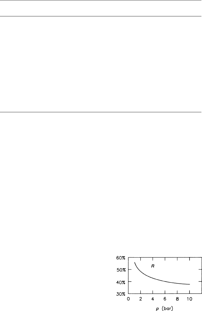
The density dependence is contained in the logarithmic term (1.59) and was

demonstrated in Fig. 1.20. The curve of Fig. 10.3 shows how the relativistic rise

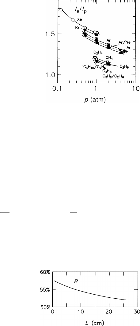
of argon goes down as the density increases. Measured ionization ratios for parti-

cles with 15 GeV/c momentum are contained in Fig. 10.4. All these data show that

the relativistic rise becomes better (higher) as the gas density is decreased and as

one passes from smaller to larger atomic numbers of the elements that make up the

gas.

The small inﬂuence of the sample length on the relativistic rise of argon is dis-

played in Fig. 10.5. The relativistic rise goes down from 57 to 53% as the sample

length increases from 1.5 to 25 cm at one bar.

Fig. 10.3 Calculated

variation of the relativistic

rise R of the most probable

ionization with the gas

density (pressure p at constant

temperature) [ALL 82]

336 10 Particle Identiﬁcation by Measurement of Ionization

Fig. 10.4 Measured ratio of

the ionization of electrons to

that of pions with momentum

of 15 GeV/c as a function of

the gas pressure for various

gases. The ionization is the

average over the lowest 40%

of 64 samples, each 4 cm long

[LEH 82b]

In a particle experiment, a determination of the ionization as a function of the

particle velocity is done with identiﬁed particles over a range of momenta. Once

the function is established it can be used for the identiﬁcation of other particles.

For this purpose it would be useful to have a mathematical description of the ion-

ization curve. Neither the theory of Bethe, Bloch, and Sternheimer nor the model

of Allison and Cobb offer a closed mathematical form. Fits have sometimes been

based on (1.66) and a piecewise parametrization of the quantity

,usingﬁveor

more parameters for

(

). Hauschild et al. have found it possible to work with

only two free parameters for

(

) and with a total of four for a description of their

data [HAU 91]. – We have sometimes used the following form for a description of

measured ionization curves:

(v)=

−

−ln





βγ



%

, (10.5)

where

= v/c,

= 1/(1 −

), and the p

are ﬁve free parameters. Equation

(10.5) is a generalization of (1.56), valid in the model of Allison and Cobb for

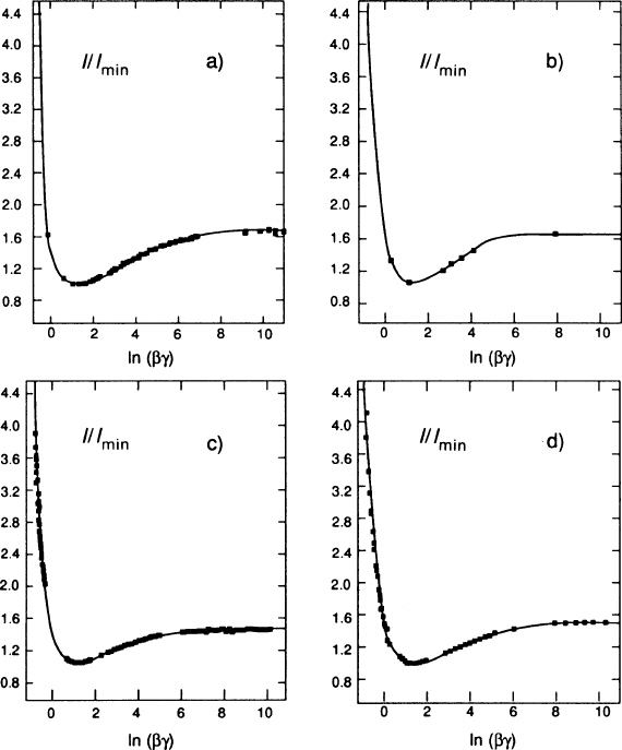
each transferred energy. Figure 10.6 shows four examples of ﬁts to this form.

Fig. 10.5 Calculated

variation of the relativistic

rise as a function of the gas

sample length for argon at

normal density [ALL 82]

10.3 Statistical Treatment of the n Ionization Samples of One Track 337

Fig. 10.6 Four different measurements of the normalized ionization strength I/I

min

ﬁttedtothe

ﬁve-parameter form (10.5) [ASS 91]. (a)DatainAr+ CH

(various small concentrations up to

10%) at 1 bar, combined from [LEH 78], [LEH 82] and ALEPH data (unpublished). (b)Datain

Ar(90%)+CH

(10%) at 1 bar [WAL 79a]. (c)DatainAr(80%)+CH

(20%) at 8.5 bar [COW 88].

(d)DatainAr(91%)+CH

(9%) at 1 bar [ALE 91]. A truncated mean was used in all cases to

measure I

10.3 Statistical Treatment of the n Ionization Samples

of One Track

The ionization measurements in the various cells, which we imagine to be of equal

size, are usually entirely independent – the transport of ionization from one cell

to its neighbour caused by the rare forward-going delta rays can be neglected,

and we exclude the effect of diffusion or electric cross-talk between neighbouring

cells. With each well-measured track we obtain n electronic signals which, up to a

338 10 Particle Identiﬁcation by Measurement of Ionization

common constant, represent n sample values of the ionization distribution in a cell.

The task is to derive from them a suitable estimator for the strength of the ionization

in the cell.

The most straightforward, the average of all n values, is a bad estimator which

ﬂuctuates a lot from track to track, because the underlying mathematical ionization

distribution has no ﬁnite average and no ﬁnite variance (see (1.33). A good estima-

tor is either derived from a ﬁt to the shape of the measured distribution or from a

subsample excluding the very high measured values.

In many cases one knows the shape of the signal distribution, f (S)dS,uptoa

scale parameter

that characterizes the ionization strength. The n signals S

,...,S

are to be used for a determination of

.Let

be ﬁxed to 1 for the normalized

reference distribution f

(S)dS. Then there is a family of normalized distributions

(S)dS =(1/

) f

(S/

)dS, (10.6)

and one must ﬁnd out which curve ﬁts best the n signal values. The most efﬁcient

method to achieve this is the maximum-likelihood method. It requires one to maxi-

mize with respect to

the likelihood function

L =

∏

(1/

) f

), (10.7)

where the product runs over all n samples. The result is a

and its error

δλ

.One

may take

to represent the most probable signal of the distribution; then

δλ

is the most probable signal measured for the track at hand.

So far, it has been assumed that the shape of the ionization curve is the same (at a

given gas length) for all ionization strengths, i.e. particle velocities. For very small

gas lengths this is not really true (see Fig. 1.21). In this case one needs a table of

different curves rather than the simple family (10.6). The rest goes as before.

For a general treatment of parameter estimation, the likelihood method, or the

concept of efﬁciency, the reader is referred to a textbook on statistics, e.g. Cram

[CRA 51] or Fisz [FIS 58] or Eadie et al. [EAD 71].

If one does not know the shape of the signal distribution beforehand, one may

use a simpliﬁed method, the method of “the truncated mean”. It is characterized by

a cut-off parameter

between 0 and 1. The estimator S

for the signal strength is

the average of the

n lowest values among the n signals S

S

∑

where m is the integer closest to

n, and the sum extends over the lowest m elements

of the ordered full sample (S

≤ S

j+1

for all j = 1,...,n −1). The quantity that

matters is the ﬂuctuation of S

divided by its value; if for a typical ionization

distribution one simulates with the Monte Carlo method the measurement of many

tracks in order to determine the best

, one ﬁnds a shallow minimum of this quantity

as a function of

between 0.35 and 0.75. In this range of

it is an empirical fact

that the values of S

are distributed almost like a Gaussian. In many practical

10.4 Accuracy of the Ionization Measurement 339

experiments the method of the truncated mean was the method of choice, because of

its simplicity and because the likelihood method had not given recognizably better

results. From a theoretical point of view, the likelihood method should be the best

as it makes use of all the available information.

Whatever the exact form of the estimator, we assume that it is a measure of

the amount of ionization, which obeys (10.2), and that the approximation (10.4) is

sufﬁciently well fulﬁlled for a practical analysis.

10.4 Accuracy of the Ionization Measurement

We have to understand how the accuracy of the ionization measurement of one track

varies with its length L and the number n of samples, with the nature of the gas and

with its pressure p. Since the distribution in a given gap with length x = L/n depends

only on the cluster-size distribution and on the number of primary interactions in

the gap, the ionization distribution varies with the density (or pressure at constant

temperature) in the same way as it does with x, and therefore the width W of the

distribution depends on x and p through their product xp. The relative accuracy will

therefore be of the form

= f (xp, n, gas) or g(Lp, n, gas).

10.4.1 Variation with n and x

If a track of length L is sampled on n small pieces of length x, we may expect that

the accuracy

in the determination of the most probable-value improves when

we increase n and L, keeping x ﬁxed. Different values of n may arise for tracks in

one event, depending on the number of samples lost because of overlapping tracks.

If the basic distribution of the ionization gathered in one piece x were well behaved

in the sense of having a mean and a variance – a prerequisite for an application of

the central-limit theorem of statistics – then the accuracy would become better with

increasing n and L according to the law

∼1/

√

n in the limit of large n.Itturns

out that with the very special cluster-size distribution of Chap. 1 the gain is more

like n

−0.46

for practical values of n when dealing with a maximum-likelihood ﬁt for

the most probable value [ALL 80]. Walenta and co-workers obtained n

−0.43

when

dealing with the average I

of the lowest 40% [WAL 79]. The differences in the

exponent seem to be small but they count for large n! In any event one deals here

with empirical relations that have not been justiﬁed on mathematical grounds.

If we vary L and x simultaneously, keeping n ﬁxed, we must consider how the

width of the ionization distribution changes with the size x of the individual sample.

The variation of L and x at constant n could be produced by increasing the gas

pressure in a suitable multiwire drift chamber.

340 10 Particle Identiﬁcation by Measurement of Ionization

As the gap is made larger, W decreases. This has been treated in Chap. 1 (see the

discussion around (1.37) and Fig. 1.10). The experiments suggest a power behaviour

of the relative width W on a single gap, which varies like

(W/I

)

: (W/I

)

=[(px)

: (px)

]

=[(pL)

: (pL)

]

(10.8)

= most probable ionization). Based on the PAI model and supported by experi-

mental data one ﬁnds that k = −0.32 [ALL 80].

Next we keep the length L = nx ﬁxed and increase n, reducing x. Now there is a

net gain in the accuracy

I proportional to

−0.14

or n

−0.11

because the better accuracy from the increase of n is partly offset by the worsening

from the decrease in x.

Although there is agreement between the different authors about these facts,

they disagree about the question down to what subdivision this rule holds. Whereas

Allison and Cobb, on the basis of their theory and in accordance with the above, rec-

ommend sampling the ionization as ﬁnely as possible [ALL 80], Walenta suggests

that below 5 cm bar in argon the improvement is negligible [WAL 79]. Lehraus et

al., from a more practical point of view, argue similarly [LEH 82a]. It must be said

that, at the time, such ﬁne samples had not been systematically explored. More re-

cently the ALEPH and the DELPHI TPCs, working at normal gas density and with

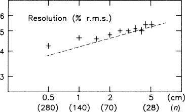
4 mm sense-wire spacing, sample remarkably thin gas layers. Figure 10.7 shows an

ALEPH study [ASS 90] in which lepton tracks from e

−

interactions were an-

alyzed by adding the signals from neighbouring sense wires, thus varying n and

x at ﬁxed L. Though not quite reaching the theoretical prediction (see below), the

measured accuracy as a function of n lends some support to the idea that ﬁne subdi-

visions down to half a cm bar may still increase the accuracy.

10.4.2 Variation with the Particle Velocity

We have seen how the single-gap width W is reduced by multiple measurements.

The value of W itself results from the summation over the cluster-size distribution

Fig. 10.7 Ionization

resolution at constant track

length as a function of the

sample length. Crosses:

measured in the ALEPH-TPC

(average track length 140 cm,

argon (91%) + methane (9%)

at 1 bar, diffusion < 1.4 mm

r.m.s.). Line:predictionof

Allison and Cobb, our (10.9)