Blank B.E., Krantz S.G. Calculus: Single Variable
Подождите немного. Документ загружается.


Thus in Example 9, T
2
(x) 5 T
1
(x) 1 2x
2
5 (1 1 2x) 1 2x
2
and T
3
(x) 5 T
2
(x) 1
4
3
x
3
5
(1 1 2x 1 2x
2
) 1
4
3
x
3
.
⁄ EXAMPLE 10 Find the Taylor polynomial of order two for the function
f (x) 5 arctan(x) about the point c 521.
Solution We
begin by calculating
f ð21Þ 52
π
4
f
ð1Þ
ð21Þ 5
1
1 1 x
2
x521
5
1
2
f
ð2Þ
ð21Þ 5
22x
ð1 1 x
2
Þ
2
x521
5
1
2
:
Therefore
T
2
ðxÞ5
2π=4
0!
ðx 1 1Þ
0
1
1=2
1!
ðx 1 1Þ
1
1
1=2
2!
ðx 1 1Þ
2
52
π
4
1
1
2
ðx 1 1Þ1
1
4
ðx 11Þ
2
:
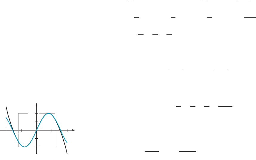
The plots of f and T
2
are shown in Figure 4. ¥
INSIGHT
Notice that the Taylor polynomial for arctan (x) that is calculated in
Example 10 does not agree with the first few terms of the Taylor series for arctan (x)in
formula (8.7.3b). The reason is that c 5 0 is the base point of expansion (8.7.3b), whereas
c 521 is the base point used in Example 10.
QUICK QUIZ
1. If f ðxÞ5
P
N
n51
x
n
=n
2
, what is f wð0Þ?
2. What is the coefficient of (x 2 9)
2
in the Taylor series of
ffiffiffi
x
p
with base point 9?
3. What is the coefficient of x
3
in the Maclaurin series of e
2x
?
4. What is the order 4 Taylor polynomial of 1/(1 1 x
2
) with base point 0?
Answers
1. 2/3 2. 21/216
3. 21/6 4. 1 2 x
2
1 x
4
T
2
(x)
arctan
(
x
)
3
y
x
2
1
m Figure 4
EXERCISES
Problems for Practice
c In each of Exercises 1210, express the given function as a
power series in x with base point 0. Calculate the radius of
convergence R. b
1.
1
1 2 2x
2.
x
1 1 x
3.
1
2 2 x
4.
1
1 1 x
2
5.
1
4 1 x
6.
1
9 2 x
2
7.
x
2
1 1
1 2 x
2
8.
x
1 1 x
2
8.7 Representing Functions by Power Series 695

9.
x
3
1 1 x
4
10.
1
16 2 x
4
c In each of Exercises 11216, use formula (8.7.2) to
express the given function as a power series in x with
base point 0. State the radius of convergence R.
b
11. ln(1 1 4x)
12. ln(5 1 2x)
13. ln(1 1 x
2
)
14. x ln(1 1 x
2
)
15.
R
x
0
lnð1 1 t
2
Þdt
16.
R
x
0
t lnð1 1 tÞdt
c
In each of Exercises 17220, use the equation (8.7.3)
to express the given function as a power series in x with
base point 0. State the radius of convergence R.
b
17. arctan
(x
2
)
18.
R
x
0
arctanðtÞdt
19.
R
x
0
arctanðt
2
Þdt
20.
R
x
0
t arctanðtÞdt
c
In each of Exercises 21226, a function f and a point
c are given. Use the equation
1
1 2 ðt 2 cÞ
5
X
N
n50
ðt 2 cÞ
n
; jt 2 cj, 1;
together with some algebra, to express f (x) as a power series
with base point c. State the radius of convergence R. b
21. f ðxÞ5
1
6 2 x
c 5 5
22. f ðxÞ5
1
x
c 5 1
23. f ðxÞ5
1
x 1 1
c 523
24. f ðxÞ5
1
x 2 4
c 5 1
25. f ðxÞ5
1
2x 1 5
c 521
26. f ðxÞ5
1
x
c 5 2
c
In Exercises 272 38, compute the Taylor polynomial
T
N
of the given function f with the given base point c
and given order N.
b
27. f ðxÞ5 cosðxÞ N 5 4 c 5 π=3
28. f ðxÞ5 sinðxÞ N 5 5 c 5 π=2
29.
f ðxÞ5
ffiffi
ffi
x
p
N 5 3 c 5 4
30. f ðxÞ5 e
2x
N 5 5 c 5 0
31.
f ðxÞ5 5x
2
1
1
x
N 5 4 c 5 1
32. f ðxÞ5 sinð3xÞ N 5 4 c 5 π=6
33.
f ðxÞ5 1=x
3
N 5 3 c 5 2
34.
f ðxÞ5 x
2
1 1 1 1=x
2
N 5 5 c 521
35. f ðxÞ5 lnð3x 1 7Þ N 5 4 c 522
36.
f ðxÞ5 e
x12
=xN5 2 c 522
37. f ðxÞ5 tanðxÞ N 5 3 c 5 0
38. f ðxÞ5 secðxÞ N 5 3 c 5 0
Further Theory and Practice
c In each of Exercises 39242, compute the Taylor polynomial
T
3
(x) of the given function f with the given base point c. b
39.
f ðxÞ5
x
x
2
1 1
c 5 1
40. f ðxÞ5 x e
x
c 5 0
41.
f ðxÞ5 ðx 1 5Þ
1=3
c 5 3
42.
f ðxÞ5 ð1 1 xÞ
1=2
c 5 2
c For each function f gi
ven in Exerci ses 43246,usetheequation
d
dx
1
1 2 x
5
1
ð1 2 xÞ
2
to find the power series of f (x)withbasepoint0. ¥
43. f (x) 5 1/(1 2 x)
2
44. f (x) 5 1/(1 2 2x)
2
45. f (x) 5 (2 1 x)/(1 2 x)
2
46. f (x) 5 1/(1 2 x)
3
c In each of Exercises 47252, find the sum of the given series in
closed form. State the radius of convergence R. b
47.
P
N
n50
x
n12
48.
P
N
n51
nx
n11
49.
P
N
n51
nðn 1 1Þx
n
50.
P
N
n52
nðn 2 1Þx
n22
51.
P
N
n51
nx
2n11
52.
P
N
n50
nðx 1 2Þ
n
c In each of Exercises 53258, use the Uniqueness Theorem to
determine the coefficients {a
n
} of the solution yðxÞ5
P
N
n50
a
n
x
n
of the given initial value problem. b
53. dy=dx 5 yyð0Þ5 1
54.
dy=dx 5 2yyð0Þ5 3
55. dy=dx 5 x 1 yyð0Þ5 1
56. dy=dx 5 2x 2 yyð0Þ5 1
57. dy=dx 5 1 1 x 1 yyð0Þ5 0
58. dy=dx 5 x 1 xy
yð0Þ5 0
c
If f ðxÞ5
P
N
n50
a
n
x
n
and gðxÞ5
P
N
n50
b
n
x
n
converge on
(2R, R), then we may formally multiply the series as though
they were polynomials. That is, if h(x) 5 f (x)g( x), then
hðxÞ5
X
N
n50
X
n
k50
a
k
b
n2k
x
n
:
The product series, which is called the Cauchy product, also
converges on (2R, R). Exercises 59262 concern the Cauchy
product. ¥
696 Chapter
8 Infinite Series

59. Suppose jxj, 1. Calculate the power series of h(x) 5
1/(1 2 x)
2
with base point 0 by using the method of Exercise
43. Using f (x) 5 g(x) 5 1/(1 2 x) 5
P
N
n50
x
n
, verify the
Cauchy product formula for h 5 f g up to the x
6
term.
60. Suppose jxj, 1. Calculate the power series of h(x) 5 1/
(1 2 x
2
) with base point 0 by substituting t 5 x
2
the
equation 1/(1 2 t) 5
P
N
n50
t
n
. Let f (x) 5 1/(1 2 x) and
g(x) 5 f (2x). Verify the Cauchy product formula for
h 5 f g up to the x
8
term.
61. The secant function has a known power series expansion
that begins
secðxÞ5 1 1
1
2
x
2
1
5
24
x
4
1
61
720
x
6
::::
The sine function has a known power series expansion
that begins
sinðxÞ5 x 2
x
3
3!
1
x
5
5!
2
x
7
7!
::::
The tangent function has a known power series expansion
that begins
tanðxÞ5 x 1
1
3
x
3
1
2
15
x
5
1
17
315
x
7
1
Verify the Cauchy product formula for tan (x) 5 sin(x)
sec (x) up to the x
7
term.
62. Suppose that the series
P
N
n50
a
n
x
n
converges on (2R, R)
to a function f (x) and that jf (x)j$ k . 0 on that interval
for some positive constant k. Then, 1/f (x) also has a
convergent power series expansion on (2R, R). Compute
its coefficients in terms of the a
n
’s. Hint: Set
1
f ðxÞ
5 gðxÞ5
X
N
n50
b
n
x
n
:
Use the equation f (x) g(x) 5 1 to solve for the b
n
’s.
Calculator/Computer Exercises
63. Let f (x) 5 (x 1 1)
4
/(x
4
1 1). It is known that f has a power
series expansion of the form
f ðxÞ5 1 1 4x 1 6x
2
1 4x
3
2 4x
5
2 6x
6
2 4x
7
1 4x
9
1
a. Plot the central difference quotient approximation
D
0
f (x,10
25
)off uðxÞ for 20.5 , x , 0.5. Use the given
power series to find a degree 8 polynomial approx-
imation of f uðxÞ. Add the plot of this polynomial to the
viewing rectangle.
b. Repeat part a but plot for 23/4 , x , 3/4. Notice that
the approximation becomes less accurate as the dis-
tance betwen x and 0, the base point of the given
series, increases.
64. Let fðxÞ5
ffiffiffiffiffiffiffiffiffiffiffiffiffi
5 1 x
2
p
. It is known that f has a power series
expansion of the form
f ðxÞ 5 3 1
2
3
ðx 2 2Þ1
5
54
ðx 2 2Þ
2
2
5
243
ðx 2 2Þ
3
1
55
17496
ðx 2 2Þ
4
1
Plot the central difference quotient approximation
D
0
f (x,10
25
)off uðxÞ for 0 , x , 4. Use the given power
series to find a degree 3 polynomial approximation T(x)
of f uðxÞ. Plot the central difference quotient approxima-
tion D
0
f (x,10
25
)off uðxÞ for 0 , x , 4. To this viewing
window, add the plot of T(x).
65. Consider the initial value problem
dy
dx
5 x
2
1 y; yð0Þ5 1:
a. Calculate the power series expansion
yðxÞ5
P
N
n50
a
n
x
n
of the solution up to the x
7
term.
b. Using the coefficients you have calculated, plot
S
3
ðxÞ5
P
3
n50
a
n
x
n
in the viewing rectangle [23, 3] 3
[211, 44].
c. The exact solution to the initial value problem is
y(x) 5 3e
x
2 x
2
2 2x 2 2, as can be determined using
the methods of Section 7.7 in Chapter 7. Add the plot
of the exact solution to the viewing window. From the
two plots, we see that the approximation is fairly
accurate for 21 # x # 1, but the accuracy decreases
outside this subinterval.
d. When a partial sum S
N
(x) is used to approximate an
infinite series, an increase in the value of N requires
more computation, but improved accuracy is the
reward. To see the effect in this example, replace the
graph of S
3
(x) with that of S
7
(x).
66. Consider the initial value problem
dy
dx
5 2 2 x 2 y; yð0Þ5 1:
a. Calculate the power series expansion
yðxÞ5
P
N
n50
a
n
x
n
of the solution up to the x
7
term.
b. Using the coefficients you have calculated, plot
S
3
ðxÞ5
P
3
n50
a
n
x
n
in the viewing rectangle [22,2] 3
[210, 1.7].
c. The exact solution to the initial value problem is
y(x) 5 32x 2 2e
2x
, as can be determined using the
methods of Section 7.7 (in Chapter 7). Add the plot of
the exact solution to the viewing window. From the
two plots, we see that the approximation is fairly
accurate for 21 # x # 1, but the accuracy decreases
outside this subinterval.
d. To see the improvement in accuracy that results from
using more terms in a partial sum, replace the graph of
S
3
(x) with that of S
7
(x).
8.7 Representing Functions by Power Series 697

8.8 Taylor Series
In the preceding section, we associated Taylor series and Taylor polynomials to a
differentiable function f. In this section, we explore two basic, related questions:
How well do the Taylor polynomials app roximate f, an d how can we tell when a
Taylor series converges to f?
Taylor’s Theorem If f is defined on an open interval centered at c, and if T
N
(x) is the order N Taylor
polynomial of f with base point c, then we define a function R
N
by
R
N
ðxÞ5 f ðx Þ2 T
N
ðxÞ: ð8:8:1Þ
Rearranging this equation, we obtain
f ðxÞ5 T
N
ðxÞ1 R
N
ðxÞ: ð8:8:2Þ
From this viewpoint, R
N
(x) is said to be a remainder term,orerror term: it is what
we must add to the approximation T
N
(x) to obtain the exact value of f (x). The key
to understanding how the Taylor polynomial T
N
can be used to approximate f is to
obtain a formula for R
N
(x) that we can analyze and estimate. Such a formula is
provided by Taylor’s Theorem.
THEOREM 1
(Taylor’s Theorem) For any natural number N, suppose that f is
N 1 1 times continuously differentiable on an open interval I centered at c.
Define R
N
(x) by equation (8.8.1). If x is a point in I, then there is a number s
between c and x such that
R
N
ðxÞ5
f
ðN11Þ
ðsÞ
ðN 1 1Þ!
ðx 2 cÞ
N11
: ð8:8:3Þ
By combining equations (8.8.2) and (8.8.3), we obtain
f ðxÞ5 T
N
ðxÞ1
f
ðN11Þ
ðsÞ
ðN 1 1Þ!
ðx 2 cÞ
N11
: ð8:8:4Þ
Compare this equation with equation (8.7.11):
T
N11
ðxÞ5 T
N
ðxÞ1
f
ðN11Þ
ðcÞ
ðN 1 1Þ!
ðx 2 c Þ
N11
:
We see that the remainder R
N
(x) is similar to the term that must be added to the
order N Taylor polynomial T
N
(x) to obtain the Taylor polynomial T
N11
(x) of one
order higher. The difference is that the derivative f
(N11)
that appears in the for-
mula for R
N
is not evaluated at the base point c,asitisinT
N11
, but at some other,
unspecified point s.
Because the order 0 Taylor polynomial T
0
(x)off is the constant function f (c),
equation (8.8.4) with N 5 0 tells us that there is a point s between c and x such that
698 Chapter 8 Infinite Series

f ðxÞ5 T
0
ðxÞ1
f
ð1Þ
ðsÞ
1!
ðx 2 cÞ
1
5 f ðcÞ1 f uðsÞðx 2 cÞ;
or
f uðsÞ 5
f ðxÞ2 f ðcÞ
x 2 c
:
This is precisely the assertion of the Mean Value Theorem. For this reason,
Taylor’s Theorem may be seen as a generalization of the Mean Value Theorem. A
proof is outlined in Exercise 80 for N 5 1 and in Exercise 81 for the general case.
⁄ EX
AMPLE 1 For f (x) 5
ffiffiffi
x
p
and c 5 1, calculate the error R
1
(4/9) that
results when T
1
(4/9) is used to approximate f (4/9). Verify formula (8.8.3) for N 5 1
and x 5 4/9.
Solution We
calculate
f ðxÞ5 1; f
ð1Þ
ðcÞ5
d
dx
ffiffiffi
x
p
x5c
5
1
2
ffiffiffi
x
p
x51
5
1
2
; and f
ð2Þ
ðcÞ5
d
2
dx
2
ffiffiffi
x
p
x5c
52
1
4x
3=2
x51
52
1
4
:
Therefore we have
T
1
ðxÞ5 f ðcÞ1
f
ð1Þ
ðcÞ
1!
ðx 2 cÞ
1
5 1 1
1
2
ðx 2 1Þ ;
which results in the approximation
T
1
4
9
5 1 1
1
2
4
9
2 1
5
13
18
of f (4/9) 5 2/3. The error R
1
(4/9) is given by
R
1
4
9
5 f
4
9
2 T
2
4
9
5
2
3
2
13
18
52
1
18
: ð8:8:5Þ
Because f
(2)
(x) 521/(4x
3/2
), equation (8.8.3) tells us that
R
1
ðxÞ5
f
ð2Þ
ðsÞ
2!
ðx 2 1Þ
2
52
1
8 s
3=2
ðx 2 1Þ
2
for some s between 1 and x. To verify this equation for x 5 4/9, we must show that
2
1
18
5
ð8:8:5Þ
R
1
4
9
52
1
8 s
3=2
4
9
2 1
2
52
25
648
1
s
3=2
has a solution s in the interval (4/9, 1). We solve the equation for s, obtaining
s 5 (25/36)
2/3
5 0.784 . . . , which is, indeed, in (4/9, 1 ). ¥
⁄ EXAMPLE 2 Calculate the order 7 Taylor polynomial T
7
(x) with base
point 0 of sin( x ). If T
7
(x) is used to approximate sin(x) for 21 # x # 1, what
accuracy is guaranteed by Taylor’s Theorem?
8.8 Taylor Series 699
Solution We first calculate
f ð0Þ5 sinð0Þ5 0
f
ð1Þ
ð0Þ5 cosðxÞj
x50
5 1
f
ð2Þ
ð0Þ52sinðxÞj
x50
5 0
f
ð3Þ
ð0Þ52cosðxÞj
x50
521
f
ð4Þ
ð0Þ5 sinðxÞj
x50
5 0
f
ð5Þ
ð0Þ5 cosðxÞj
x50
5 1
f
ð6Þ
ð0Þ52sinðxÞj
x50
5 0
f
ð7Þ
ð0Þ52cosðxÞj
x50
521
f
ð8Þ
ðxÞ5 sinðxÞ:
Therefore
T
7
ðxÞ 5
0
0!
ðx 2 0Þ
0
1
1
1!
ðx 2 0Þ
1
1
0
2!
ðx 2 0Þ
2
1
ð21Þ
3!
ðx 2 0Þ
3
1
0
4!
ðx 2 0Þ
4
1
1
5!
ðx 2 0Þ
5
1
0
6!
ðx 2 0Þ
6
1
ð21Þ
7!
ðx 2 0Þ
7
5 x 2
x
3
3!
1
x
5
5!
2
x
7
7!
:
The remainder term is given by
R
7
ðxÞ5
f
ð8Þ
ðsÞ
8!
ðx 2 0Þ
8
5
sinðsÞ
8!
x
8
:
Thus
sinðxÞ5 x 2
x
3
3!
1
x
5
5!
2
x
7
7!
1
sinðsÞ
8!
x
8
for some value of s between 0 and x. Because jsin(s)j can be no greater than 1 and
1/8! , 0.000025, we can make the estimate
jR
7
ðxÞj5
sinðsÞ
8!
x
8
#
jsinðsÞj
8!
, 0:000025 for jxj# 1:
Therefore sin(x)andx 2 x
3
/3! 1 x
5
/5!2x
7
/7! agree to four decimal places when
jxj# 1. As Figure 1 shows, x 2 x
3
/3! 1 x
5
/5! 2 x
7
/7! is a good approximation of sin(x)
on an even larger interval.
¥
⁄ EXAMPLE 3 Calculate the order 4 Taylor polynomial T
4
(x) with base
point π/4 of sin(x). If T
4
(x) is used to approximate sin(x) for 0 # x # π/2, what
accuracy is guaranteed by Taylor’s Theorem?
Solution Using
the derivatives calculated in the preceding example, we have
f ðπ=4Þ5 1=
ffiffiffi
2
p
, f
ð1Þ
ðπ=4Þ5 cosðπ=4Þ5 1=
ffiffiffi
2
p
, f
ð2Þ
ðπ=4Þ52sinðπ=4Þ521 =
ffiffiffi
2
p
,
f
ð3Þ
ðπ=4Þ52cosðπ=4Þ521=
ffiffiffi
2
p
, f
ð4Þ
ðπ=4Þ5 sinðπ=4Þ5 1=
ffiffiffi
2
p
, and f
ð5Þ
ðxÞ5 cosð x Þ.
Therefore
y sin(x)
y
x
244
1.0
0.5
y x
x
3
3!
x
5
5!
x
7
7!
2
m Figure 1
700 Chapter
8 Infinite Series

T
4
ðxÞ5
1=
ffiffiffi
2
p
0!
x 2
π
4
0
1
1=
ffiffiffi
2
p
1!
x 2
π
4
1
2
1=
ffiffiffi
2
p
2!
x 2
π
4
2
2
1=
ffiffiffi
2
p
3!
x 2
π
4
3
1
1=
ffiffiffi
2
p
4!
x 2
π
4
4
;
or
T
4
ðxÞ5
1
ffiffiffi
2
p
1
1
ffiffiffi
2
p
x 2
π
4
2
1
2!
ffiffiffi
2
p
x 2
π
4
2
2
1
3!
ffiffiffi
2
p
x 2
π
4
3
1
1
4!
ffiffiffi
2
p
x 2
π
4
4
:
According to formula (8.8.3), the remainder is given by
R
4
ðxÞ5
f
ð5Þ
ðsÞ
5!
x 2
π
4
5
5
cosðsÞ
5!
x 2
π
4
5
;
where s is between π/4 and x. Because jx 2 π/4j# π/2 2 π/4 5 π /4 5 0.785398 . . . and
cos(s) # 1 , we have
jR
4
ðxÞj5
jf
ð5Þ
ðsÞj
5!
x 2
π
4
5
#
1
5!
ð0:785398:::Þ
5
, 0:0025:
Thus for x in the interval [0, π/2], T
4
(x) approximates sin(x) to two decimal
places.
¥
INSIGHT
As we observed in the preceding section, Taylor polynomials that are
calculated at distinct base points may look quite different. The Taylor polynomials of
sin(x) involve only odd powers of x when c 5 0 is used as the base point (Example 1).
That is not the case when the base point is π/4 (Example 2).
Estimating the
Error Term
The following theorem formalizes the method of estimation employed in Examples
1 and 2.
THEOREM 2
Let f be a function that is N 1 1 times continuously differentiable
on an open interval I centered at c. For each x in I, let J
x
denote the closed
interval with endpoints x and c. Thus J
x
5 [c, x] if c # x and J
x
5 [x, c ] if x , c. Let
M 5 max
t2J
x
jf
ðN11Þ
ðtÞj: ð8:8:6Þ
Then the error term R
N
(x) defined by equation (8.8.1) satisfies
jR
N
ðxÞj#
M
ðN 1 1Þ!
jx 2 cj
N11
: ð8:8:7Þ
Proof. Taylor’s
Theorem expresses the remainder R
N
(x) in terms of a derivative
f
(N 1 1)
(s) that is evaluated at an undetermine d point s between c and x. We bound
the remainder by using the largest possible value for this derivative. Because s
belongs to J
x
, we have
jR
N
ðxÞj5
f
ðN11Þ
ðsÞ
ðN 1 1Þ!
ðx 2 cÞ
N11
5
jf
ðN11Þ
ðsÞj
ðN 1 1Þ!
jx 2 cj
N11
#
M
ðN 1 1Þ!
jx 2 cj
N11
: ’
8.8 Taylor Series 701

⁄ EXAMPLE 4 Use the third order Taylor polynomial of e
x
with base point 0
to approximate e
20.1
. Estimate your accura cy.
Solution If f (x) 5 e
x
, then f
(k)
(x) 5 e
x
for all natural numbers k. Thus f
(k)
(0) 5 1
for k 5 0, 1, 2, 3, and
T
3
ðxÞ5
X
3
k50
f
ðkÞ
ð0Þ
k!
x
k
5 1 1 x 1
1
2!
x
2
1
1
3!
x
3
:
Our approximation is therefore T
3
(20.1) 5 1 1 (20.1) 1 (20.1)
2
/2 1 (20.1)
3
/6 5
0.90483 . . . . Next, to estimate the accuracy of this approximation, we calculate
M 5 max
2 0:1 # t # 0
d
4
dt
4
e
t
5 max
2 0:1 # t # 0
e
t
5 e
0
5 1:
Therefore
jR
3
ð2 01Þj#
1
4!
j2 01 2 0j
4
5 4166::: 3 10
26
, 5 3 10
26
:
Our error estimate guarantees that our approximation is accurate to five decimal
places. A check with a calculator shows this to be correct.
¥
INSIGHT
When jf
(N 1 1)
(t)j is a monotonic function on the interval J
x
between c
and x, as in Example 3, the maximum M 5 max
t2J
x
jf
ðN11Þ
ðtÞj occurs at an endpoint of J.
That is, M is the larger of jf
(N 1 1)
(c)j and jf
(N 1 1)
(x)j.
Achieving a D esired
Degree of Accuracy
To approxi mate the value of f (x) by the value T
N
(x) of a Taylor polynomial, we
must select a base point c and an order N. The base point c is chosen to facilitate
computation. Another important consideration is that, if jx 2 cj is small, then the
factor jx 2 cj
N11
of jR
N
(x)j will be small. Choosing a large value of N is also an
obvious strategy for producing a small error term. However, it is not advantageous
to choose a value of N that is larger than necessary. To minimize the amount of
calculation, we desire the smallest N that gives the required accuracy. Studying
several examples is the best way to understand the method of choosing values of c
and N that are appropriate for attaining a particular degree of accuracy.
⁄ EX
AMPLE 5 Compute ln(1.2) to an accuracy of four decimal places.
Solution Let f (x) 5 ln(x).
Saying that we requir e four decimal places of accuracy
means that we want the error term to be less than 5 10
25
. Thus we require
jR
N
(1.2)j, 5 10
25
. We can arrange for this estimate to be true by choosing c
sensibly and by making N sufficiently large. We take c 5 1, which is reasonably
close to 1.2, and note that, for f (x) 5 ln(x), we have f
(1)
(x) 5 x
21
, f
(2)
(x) 5
21 x
22
521! x
22
, f
(3)
(x) 5 2 x
23
5 2! x
23
, f
(4)
(x) 523 2 x
24
523! x
24
,
f
(5)
(x) 5 4! x
25
, and, in general,
f
ðnÞ
ðxÞ5 ð21 Þ
n21
ðn 2 1Þ! x
2n
n 5 1; 2 ; 3;::: : ð8:8:8Þ
702 Chapter 8 Infinite Series
Thus
f
ðnÞ
ðcÞ
n!
5
ð21Þ
n21
ðn 2 1Þ! c
2n
n!
5
ð21Þ
n21
ðn 2 1Þ! 1
2n
n!
5
ð21Þ
n21
n
and
T
N
ð1:2Þ5 lnðcÞ1
X
N
n51
f
ðnÞ
ðcÞ
n!
ð1:2 2 cÞ
n
5 lnð1Þ1
X
N
n51
ð21Þ
n21
n
ð1:2 2 1Þ
n
5
X
N
n51
ð21Þ
n21
ð0:2Þ
n
n
: ð8:8:9Þ
To estimate the error, we note that f
(N 1 1)
(t) 5 (2 1)
N
N! t
2(N 1 1)
by formula
(8.8.8). Therefore
M 5 max
1 # t # 1:2
f
ðN11Þ
ðtÞ
5 max
1 # t # 1:2
jð21Þ
N12
N! t
2ðN11Þ
j5 N! max
1 # t # 1:2
1
t
N11
5 N!
(because the maximum of 1/t
N11
for 1 # t # 1.2 occurs at t 5 1). Thus
jR
N
ð1:2Þj# M
j1:2 2 1j
N11
ðN 1 1Þ!
5 N!
ð0:2Þ
N11
ðN 1 1Þ!
5
ð0:2Þ
N11
N 1 1
:
To ensure that the error is less than 5 10
25
, it suffices to choose N large enough so
that (0.2)
N11
/(N 1 1) , 5 10
25
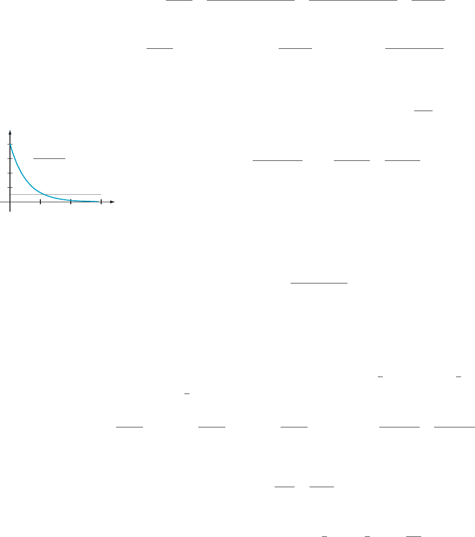
. Substituting in a few values for N, we see that the
inequality will first be true when N 5 5. We could also determine this value of N by
plotting (0.2)
N 1 1
/(N 1 1), as in Figure 2.
In conclusion, the formula ln(1.2) 5 T
5
(1.2) 1 R
5
(1.2) and the inequality
jR
5
(1.2)j, 5 10
25
assure us that ln(1.2) and T
5
(1.2) agree to four decimal places.
Substituting N 5 5 in line (8.8.9), we calculate
lnð1:2ÞT
5
ð1:2Þ5
X
5
n51
ð21Þ
n21
ð0:2Þ
n
n
5 0:1823:::: ¥
⁄ EX
AMPLE 6 In Example 1 of Section 3.9 of Chapter 3, we used the dif-
ferentia
l approximation to calculate three decimal places of
ffiffiffiffiffiffiffi
4:1
p
. How many
decimal places of accuracy are obtained by using a second order Taylor polynomial
to approximate
ffiffiffiffiffiffiffi
4:1
p
?
Solution Let f (x) 5
ffiffi
ffi
x
p
and c 5 4. We calculate f
(1)
(x) 5
1
2
x
21/2
, f
(2)
(x) 52
1
4
x
23/2
,
and f
(3)
(x) 5
3
8
x
25/2
. Using the first two of these derivatives, we obtain
T
2
ð4:1Þ5
f
ð0Þ
ð4Þ
0!
ð4:1 2 4Þ
0
1
f
ð1Þ
ð4Þ
1!
ð4:1 2 4Þ
1
1
f
ð2Þ
ð4Þ
2!
ð4:1 2 4Þ
2
5 2 1
ð4:1 2 4Þ
4
2
ð4:1 2 4Þ
2
64
;
or
T
2
ð4:1Þ5 2 1
ð0:1Þ
4
2
ð0:1Þ
2
64
5 2:02484375 :
Using the last calculated derivative, f
(3)
(x) 5 (3/8)x
25/2
, we have
M 5 max
4 # t # 4:1
f
ð3Þ
ðtÞ
5 max
4 # t # 4:1
3
8
t
25=2
5
3
8
4
25=2
5
3
256
:
N
0.0004
0.0003
456
0.0002
0.0001
y
y 5 10
5
y
(0.2)
N1
N 1
m Figure 2
8.8 Taylor Series 703

Therefore
jR
2
ð4:1Þj#
M
3!
ð4:1 2 4Þ
3
5
3
256 3!
ð0:1 Þ
3
5 1:953125 3 10
26
, 5 3 10
26
:
Thus T
2
(4.1) 5 2.02484375 approximates
ffiffiffiffiffiffiffi
4:1
p
with an error less that 5 3 10
26
.In
other words, our approximation is accurate to five decimal places.
¥
Taylor Series
Expansions of the
Common
Transcendental
Functions
Suppose that f is infinitely differentiable on an open interval centered at c. We can
then form the Taylor series
TðxÞ5
X
N
n50
f
ðnÞ
ðcÞ
n!
ðx 2 cÞ
n
ð8:8:10Þ
of f. (Recall that the term Maclaurin series is also used when c 5 0.) Let R denote
the radius of convergence of this series and suppose that R . 0. From Section 8.7,
we know that T(x) is the only power series with base point c that can represent f on
the open interval I 5 (c 2 R, c 1 R). Whether T(x)isf (x) or another function is the
subject of the next theorem.
THEOREM 3
Suppose that f is infinitely differentiable on an interval containing
points c and x. Let R
N
(x) be defined by equation (8.8.1). Then
TðxÞ5 lim
N-N
X
N
n50
f
ðnÞ
ðcÞ
n!
ðx 2 c Þ
n
exists if and only if lim
N-N
R
N
ðxÞ exists and
f ðxÞ5
X
N
n50
f
ðnÞ
ðcÞ
n!
ðx 2 c Þ
n
if and only if
lim
N-N
R
N
ðxÞ5 0:
Proof. We
let N tend to infinity in equation (8.8.2). The result is
f ðxÞ5 lim
N-N
T
N
ðxÞ1 R
N
ðxÞ
5 lim
N-N
X
N
n50
f
ðnÞ
ðcÞ
n!
ðx 2 cÞ
n
1 R
N
ðxÞ
;
from which both assertions follow. ’
In Section 8.7, we calc ulated power series expan sions of ln(1 1 x),
arctan(x),
and a few other functions. Now we will use Theorem 3 to do the same for some
other basic functions. Before we attack some concrete examples, we must first
compute the limit of a certain sequence that will occur in most of our examples.
THEOREM 4
If b is a fixed positive constant, then
lim
k-N
b
k
k!
5 0: ð8:8:11Þ
704 Chapter 8 Infinite Series