Blank B.E., Krantz S.G. Calculus: Single Variable

Подождите немного. Документ загружается.

59. [α, β)

60. [α, β]

61. Is it possible for a power series to have interval of con-

vergence (2N, 1)? Could it have interval of convergence

(0,N)? Explain your answers.

62. What is the radius of convergence of

n51

n! ðx=nÞ

63. Let a

k51

1=k

. What is the radius of convergence of

n51

64. Let b

k51

ﬃﬃﬃ

. What is the radius of convergence

n51

65. Suppose that a

6¼0 for n $ 0. Show that if

‘ 5 lim

n-N

n11

j=ja

j exists (as a nonnegative number or

N), then R 5 1/‘ is the radius of convergence of

n50

. Hint: Follow Examples 6 and 7, and apply the

Ratio Test to the series

n50

where u

5 a

66. Let a

5 1, a

5 0, a

5 3

, a

5 a

5 0, a

5 6

, a

5 a

5 0, a

5 10

210

, and, in general, a

5 N

if N 5

n(n 1 1)/2 for some positive integer n and a

5 0 otherwise.

Calculate the radius of convergence of

n50

67. For each odd positive integer n, let a

5 n. For each even

positive integer n, let a

5 2a

n21

. Calculate the radius of

convergence of

n51

Calculator/Computer Exercises

68. We know the validity of the equation

n50

ð21Þ

1=ð1 1 xÞ for 21 , x , 1. In this exercise, we will explore

this equation by graphing partial sums S

ðxÞ5

n50

ð21Þ

n50

ð21Þ

for several values of N.

a. Plot f (x) 5 1/(1 1 x) for 20.6 , x , 0.6. In the same

window, ﬁrst add the plot of S

(x), then the plot of

(x), and ﬁnally S

(x). You will notice the increasing

accuracy as N increases. In this window, the graphs of

(x) and f (x) would not be distinguishable because

the functions agree to four decimal places.

b. Repeat part a but plot over the interval 0.6 , x , 0.95.

Notice that the convergence of S

(x) is less rapid as x

moves away from the center 0 of the interval of con-

vergence. If you are working with a computer algebra

system, replace the plot of S

(x) with a plot of S

(x). You

will see that, for x in the interval of convergence but near

an endpoint, S

(x) can be used to accurately approximate

f (x), but a large value of N mayberequired.

c. Repeat part a but plot over the interval 20.98 , x ,

20.6. Here the problem is that the function f (x) has a

singularity at the left endpoint 21 of the interval of

convergence of the power series.

69. We know the validity of the equation

n50

5 1=ð1 2 xÞ

for 21 , x , 1. In this exercise, we will explore this

equation by graphing partial sums S

ðxÞ5

n50

for several values of N.

a. Plot f (x) 5 1/(1 2 x) for 20.6 , x , 0.6. In the same

window, ﬁrst add the plot of S

(x), then the plot of

(x), and ﬁnally S

(x). You will notice the increasing

accuracy as N increases. In this window, the graphs of

(x) and f (x) would not be distinguishable because

the functions agree to four decimal places.

b. Repeat part a but plot over the interval 20.95 , x ,

20.6. Notice that the convergence of S

(x) is less rapid

as x moves away from the center 0 of the interval of

convergence. If you are working with a computer

algebra system, replace the plot of S

(x) with a plot of

(x). You will see that, for x in the interval of con-

vergence but near an endpoint, S

(x) can be used to

accurately approximate f (x), but a large value of N

may be required.

c. Repeat part a but plot over the interval 0.6 , x , 0.98.

Here the problem is that the function f (x) has a sin-

gularity at the right endpoint 1 of the interval of

convergence of the power series.

70. It is known that the equation

n50

5 x =ðx 2 1Þ

holds

for 21 , x , 1. In this exercise, we will explore this

equation by graphing partial sums S

ðxÞ5

n50

for several values of N.

a. Plot f (x) 5 x/(x 2 1)

for 20.5 , x , 0.5. In the same

window, ﬁrst add the plot of S

(x), then the plot of

(x), and ﬁnally S

(x). You will notice the increasing

accuracy as N increases.

b. Repeat part a but plot over the interval

20.8 , x ,20.5. Notice that the convergence of S

(x)

is less rapid as x moves away from the center 0 of the

interval of convergence. If you are working with a

computer algebra system, replace the plot of S

(x)

with a plot of S

(x). You will see that, for x in the

interval of convergence but near an endpoint, S

(x)

can be used to accurately approximate f (x), but a large

value of N may be required.

c. Repeat part a but plot over the interval 0.5 , x , 0.9. If

you are working with a computer algebra system,

replace the plot of S

(x) with a plot of S

(x).

71. We know that

n50

ð21Þ

5 1=ð1 1 tÞ for 21 , t , 1.

Therefore for 21 , x , 1, we have

lnð1 1 xÞ5

1 1 t

dt 5

n50

ð21Þ

dt:

In this exercise, we will investigate graphically the

approximation that results when an inﬁnite series is

truncated and then integrated term by term.

a. Plot f (x) 5 ln(1 1 x) for 20.5 # x # 1. In the same

window, ﬁrst add the plot of S

ðxÞ5

n50

ð21Þ

dt for N 5 2, then the plot of S

(x),

and ﬁnally S

(x). You will notice the increasing accu-

racy as N increases. In this window, the graphs of

(x) and f (x) would be distinguishable only at the

rightmost few pixels.

b. Repeat part a but plot over the interval 20.99 , x ,

20.5. Here the problem is that the function f (x) has a

8.6 Introduction to Power Series 685

singularity at the left endpoint 21 of the interval of

convergence of the power series. Still, accuracy in the

interval of convergence can be attained by increasing

the value of N. If you are working with a computer

algebra system, replace the plot of S

(x) with a plot of

(x).

8.7 Representing Functions by Power Series

A natural question to ask is, if a power series deﬁnes a function, can we always say

what funct ion it is? The answer is, No. Most functions, those deﬁned by power

series included, do not have familiar names. A more fruitful question is, can we

write the functions with which we are familiar as power series? The answer to this

question is, with certain restrictions, Yes. Beginning with this section, we will study

how to go back an d forth between functions and power series.

Power Series

Expansions of Some

Standard Functions

For each ﬁxed x, the power series

n50

can be regarded as a geometric series.

Because we know that this series converges to 1/(1 2 x)ifx belongs to the interval

(21, 1), we have

1 2 x

n50

5 1 1 x 1 x

1 x

1  ð21 , x , 1Þ:

This formula can be used to ﬁnd power series representations for many functions

that are related to 1/(1 2 x). To facilitate substitution, we rewrite this equation with

a different variable:

1 2 u

n50

5 1 1 u 1 u

1 u

1  ð21 , u , 1Þ: ð8:7:1Þ

⁄ EX

AMPLE 1 Express

ð4 1 x

by means of a power series with base point 0.

Solution The

key idea is to rewrite the denominator of the given function in the

form 1 2 u and then use formula (8.7.1). We accomplish this manipulation by

writing

4 1 x



1 2 ð2x

=4Þ



ð1 2 uÞ

;

where u 52x

/4. If 22 , x , 2, then 21 , u , 1. Substituting u 52x

/4 in equation

(8.7.1), we obtain

4 1 x

ð1 2 uÞ

ð8:7:1Þ

n50





ð22 , x , 2Þ:

We conclude that

4 1 x

n50





n50

ð21Þ





n11

2n13

ð22 , x , 2Þ:

If we write out several terms, then this equation becomes

686 Chapter 8 Inﬁnite Series

4 1 x

256

1024

4096

|ﬄﬄﬄﬄﬄﬄﬄﬄﬄﬄﬄﬄﬄﬄﬄﬄﬄﬄﬄﬄﬄﬄﬄﬄﬄﬄﬄﬄﬄﬄﬄﬄﬄﬄﬄﬄﬄﬄﬄﬄﬄﬄﬄﬄﬄﬄﬄﬄ{zﬄﬄﬄﬄﬄﬄﬄﬄﬄﬄﬄﬄﬄﬄﬄﬄﬄﬄﬄﬄﬄﬄﬄﬄﬄﬄﬄﬄﬄﬄﬄﬄﬄﬄﬄﬄﬄﬄﬄﬄﬄﬄﬄﬄﬄﬄﬄﬄ}

PðxÞ

1  22 , x , 2:

Figure 1 shows that the degree 13 polynomial P(x) that we obtain by truncating the

inﬁnite series is quite a good approximation to x

/(4 1 x

) for x not too far away

from the center of the interval of convergence. In the ﬁgure, the plots of x

/(4 1 x

)

and P(x) are barely distinguishable for 21.5 , x , 1.5.

⁄ EXAMPLE 2 Find a power series representation for the function F(x) 5

ln(1 1 x).

Solution The

relationship of F to formula (8.7.1) becomes apparent after

differentiation:

FuðxÞ5

lnð1 1 xÞ5

1 1 x

1 2 ð2xÞ

1 2 u

where u 52x:

For 21 , x , 1, we also have 21 , u , 1. We may therefore apply formula (8.7.1)

to obtain

FuðxÞ5

1 2 u

ð8:7:1Þ

n50

ð2xÞ

n50

ð21Þ

ð21 , x , 1Þ:

Next, we integrate both sides of this equation. Theorem 5b of Section 8.6 tells us

that the right-hand side may be integrated termwise. The result is

FðxÞ5

n50

ð21Þ

n11

n 1 1

1 C ð 21 , x , 1Þ;

where C is a constant of integration. By setting x 5 0 in this equation, we obtain

F(0) 5 C. Because F(0) 5 ln(1 1 0) 5 0, we conclude that C 5 0. Thus we have

derived the formula

lnð1 1 xÞ5

n50

ð21Þ

n11

n 1 1

ð21 , x , 1Þ:

It is not wrong to leave the series in this form, but we prefer to simplify the

exponent to which x is raised. By changing the index of summation to m 5 n 1 1, we

obtain

lnð1 1 xÞ5

m51

ð21Þ

m21

ð21 , x , 1Þ: ð8:7: 2aÞ ¥

INSIGHT

It is usually a good idea to write out the ﬁrst several terms of a new series

as a visual aid. For instance, equation (8.7.2a) becomes

lnð1 1 xÞ5 x 2

:::

for 21 , x , 1: ð8:7: 2bÞ

1.5

1.5

1.0

0.5

0.5

1.0

P(x)

4 

m Figure 1

8.7 Representing Functions by Power Series 687

⁄ EXAMPLE 3 Use formula (8.7.2b) to calculate ln(1.1) with an error no

greater than 0.0001.

Solution Formul

a (8.7.2b) tells us that

lnð1:1Þ5 lnð1 1 0:1Þ5 0:1 2

ð0:1Þ

1 

We can estimate this quantity by truncating the alternating inﬁnite series.

According to inequality (8.4.1) of the Alternating Series Test, the error that results

is less than the ﬁrst term that is omitted. Therefore

lnð1 1 0:1 Þ5 0:1 2

ð0:1Þ

1 ε

where ε is an error that is less than

(0.1)

5 0.000025 in absolute value. The

required approximation is

lnð1:1Þ0:1 2

ð0:1Þ

5 0:09533::::

A check with a calculator will verify the indicated accuracy.

⁄ EXAMPLE 4 Find a power series expansion for F(x) 5 arctan (x) that is

valid for 21 , x , 1.

Solution We

use the same idea that was the basis of Example 2. Our starting

point is

FuðxÞ5

arctanðxÞ5

1 1 x

1 2 u

where u 52x

Notice that 21 , u # 0 for 21 , x , 1. For these values of u, the geometric series

n50

converges to 1/(1 2 u). Therefore

FuðxÞ5

1 2 u

ð8:7:1Þ

n50

ð2x

n50

ð21Þ

ð21 , x , 1Þ:

Now we ﬁnd antiderivatives of both sides. The result is

arctanðxÞ5

n50

ð21Þ

2n11

2n 1 1

1 C ð 21 , x , 1Þ:

Setting x 5 0 shows that C 5 arctan(0) 5 0. Therefore

arctanðxÞ5

n50

ð21Þ

2n11

2n 1 1

ð21 , x , 1Þ; ð8:7:3aÞ

or, in a form that is more easily recogn ized and remembered,

arctanðxÞ5 x 2

2  for 21 , x , 1: ð8:7:3bÞ ¥

688 Chapter 8 Inﬁnite Series

INSIGHT

Power series representations (8.7.2b) and (8.7.3b) for ln(1 1 x) and

arctan (x) are valid for 21 , x , 1. The Alternating Series Test tells us that the series

in these formulas converge when x 5 1 as well. Because each side of equations (8.7.2b)

and (8.7.3b) makes sense for x 5 1, it is plausible to think that these equations remain

valid for x 5 1. That is,

lnð2Þ5 1 2

2  ð8:7:4Þ

and, because arctan (1) 5 π/4,

5 1 2

2  ð8:7:5Þ

In fact, both of these formulas are true. Proving them requires a delicate interchange of

limits that we will omit. Although formulas (8.7.4) and (8.7.5) are interesting, they are

not very efﬁcient from a computational viewpoint. For instance, after summing the ﬁrst

100 terms that appear on the right side of formula (8.7.5), we get

 1 2

1 2

199

5 0:7828982::::

This results in the approximation π 4 3 0.7828982 . . . 5 3.131 ..., which is correct to

only one decimal place!

Thus far, the base point used in all examples of this section has been 0. At

times, other base points may be desirable or, as in the next example, necessary.

⁄ EX

AMPLE 5 Expand 1/x and 1/x

in powers of x 2 1 for jx 2 1j, 1.

Solution First

notice that, on applying formula (8.7.1) with u 5 12 x, we have

1 2 ð1 2 xÞ

ð8:7:1Þ

n50

ð1 2 xÞ

n50

ð21Þ

ðx 2 1Þ

; jx 2 1j, 1:

Differentiating both sides of this equation, we obtai n 21=x

n51

nð21Þ

ðx 2 1Þ

n21

,or1=x

n51

nð21Þ

n21

ðx 2 1Þ

n21

for jx 2 1j, 1. To write this power

series in standard form, we set m 5 n 2 1. As n runs through the integers from 1 to

inﬁnity, the index m runs through the integers from 0 to inﬁnity. This change of

summation index gives us

m50

ð21Þ

ðm 1 1Þðx 2 1Þ

for jx 2 1j, 1:

If we write out several terms, then we obtain

5 1 2 2 ðx 2 1Þ1 3ðx 2 1Þ

2 4ðx 2 1Þ

1  for jx 2 1j, 1: ð8:7:6Þ ¥

A LOOK FORWARD c Every power series representation that we have obtained so

far has been derived from the identity 1=ð1 2 xÞ5

n50

for |x| , 1. It is sur-

prising, perhaps, that functions such as ln(1 1 x) and arctan(x) can be treated using

this approach. These examples should not, however, lead us to overestimate the

8.7 Representing Functions by Power Series 689

scope of the techniques that have been presented. Power series representations of

other important funct ions such as e

, sin(x), and cos(x) require the more general

methods that we develop in the next section.

The Relationship

between the

Coefﬁcients and

Derivatives

of a Power Series

Theorem 6 of Section 8.7 tells us that, if a power series

n50

ðx2cÞ

converges on

an open interval I centered at c,thenthefunctionf (x) deﬁned by f ðxÞ5

n50

ðx 2 cÞ

is inﬁnitely differentiable on I. In other words, the n

derivative

(n)

(c)off at c exists for every positive integer n. The next theorem tells us that the

coefﬁcient a

can be expressed in terms of f

(n)

(c). To avoid having to treat the index

n 5 0 as a special case, it will be convenient to understand f

(0)

(c)tomeanf (c).

THEOREM 1

Suppose that the power series

n50

ðx2cÞ

converges on an

open interval I centered at c. Let f be the function deﬁned on I by f ðxÞ5

n50

ðx 2 cÞ

: Then

ðnÞ

ðcÞ

; n 5 0; 1; 2; 3;::: ð8:7:7Þ

and

f ðxÞ5

n50

ðnÞ

ðcÞ

ðx 2 cÞ

: ð8:7:8Þ

Proof. Bec

ause a

5 f (c) 5 f

(0)

(c)/0!, equation (8.7.7) holds when k 5 0.

Now suppose that k is a positive integer. Observe that

ðx 2 cÞ

0ifn , k

k! if n 5 k

nðn 2 1Þðn 2 k 1 1Þðx 2 cÞ

n2k

if n . k

From the last line of this equation, we see that

ðx 2 cÞ



x5c

5 n ðn 2 1Þðn 2 k 1 1Þðc 2 cÞ

n2k

5 0

when n . k. By dividing the power series for f (x) into three parts,

f ðxÞ5

k21

n50

a ðx 2 cÞ

|ﬄﬄﬄﬄﬄﬄﬄﬄﬄﬄ{zﬄﬄﬄﬄﬄﬄﬄﬄﬄﬄ}

n,k

1 a

ðx 2 cÞ

|ﬄﬄﬄﬄﬄﬄ{zﬄﬄﬄﬄﬄﬄ}

n5k

n5k11

ðx 2 c Þ

|ﬄﬄﬄﬄﬄﬄﬄﬄﬄﬄﬄﬄ{zﬄﬄﬄﬄﬄﬄﬄﬄﬄﬄﬄﬄ}

n.k

;

and differentiating k times term by term, we see that

ðkÞ

ðxÞ5 0 1 k!  a

n5k11

nðn 2 1Þðn 2 k 1 1Þa

ðx 2 c Þ

n2k

and

ðkÞ

ðcÞ5 0 1 k!  a

1 0:

690 Chapter 8 Inﬁnite Series

Equation (8.7.7) follows. Formula (8.7.8) is then obtained by substituting the value

equation (8.7.7) gives for a

into f ðxÞ5

n50

ðx 2 cÞ

: ’

⁄ EXAMPLE 6 Let f ð x Þ5

n50

ð21Þ

ðn 1 1Þðx 2 1Þ

. What are f uð1Þ; f vð1Þ,

and f wð1Þ?

Solution The

coefﬁcients {a

} of the power series deﬁning f are given by

5 (21)

(n 1 1) for 0 # n ,N. The base point is c 5 1. Because

‘ 5 lim

n-N



n11



5 lim

n-N

n 1 2

n 1 1

5 lim

n-N

1 1 2=n

1 1 1=n

5 1;

we see that the radius of convergence R is given by R 5 1/‘ 5 1. All that is needed to

apply Theorem 1 is that R . 0. We may therefore use formula (8.7.7), which tells us

that f

(k)

. Consequently, on setting k 5 1, 2, and 3, we have f uð1Þ5

1!  a

5 1! ð21Þ

ð1 1 1Þ522; f vð1Þ5 2!  a

5 2! ð21Þ

ð2 1 1Þ5 6; and f wð1Þ5 3!

5 3! ð21Þ

ð3 1 1Þ5224: ¥

INSIGHT

Notice that the formula f

(k)

permits the calculation of f

(k)

(c)

without the beneﬁt of a closed form for f (x). However, equation (8.7.6) shows that the

power series that deﬁnes f (x) in Example 6 is equal to 1/x

. In other words, the function

f (x) of Example 6 is equal to 1/x

. We may therefore check the results of Example 6 by

directly calculating f uðxÞ522/x

, f vðxÞ5 6/x

, and f wðxÞ5224/x

. On evaluation at

x 5 1, we obtain f uð1Þ522, f vð1Þ5 6, and f wð1Þ5224, in agreement with the values

obtained by using the formula f

(k)

In Example 6, the coefﬁc ient a

of a power series representing a function f is

used to calculate f

(k)

(c). In the next example, equation (8.7.7) is applied in the

opposite direction: f

(k)

⁄ EX

AMPLE 7 The error function x/erf (x) is deﬁned by

erfðxÞ5

ﬃﬃﬃ

dt; 2N , x , N:

As its name suggests, the error function arises in the analysis of observational

errors. The error function also plays an important role in the theory of refraction

and the theory of he at conduction. It is known that the error function has a

convergent power series representation

n50

. Calcul ate the partial sum

n50

Solution Let f (x) 5 erf(x).

By the Fundamental Theorem of Calculus, we have

f uðxÞ5 ð2=

ﬃﬃﬃ

Þe

. We calculate f

ð2Þ

ðxÞ52ð4=

ﬃﬃﬃ

Þxe

and f

ð3Þ

ðxÞ5

2 ð4=

ﬃﬃﬃ

Þe

1 ð8=

ﬃﬃﬃ

Þx

. It follows that f (0) 5 0, f

(1)

(0) 5 2/

ﬃﬃﬃ

, f

(2)

(0) 5 0,

and f

(3)

(0) 524/

ﬃﬃﬃ

. We obtain the requested partial sum by setting c 5 0in

equation (8.7.8), omitting all terms with index n greater than 3, and substituting in

the computed values of f (0), f

(1)

(0), f

(2)

(0), and f

(3)

(0):

n50

ðnÞ

ð0Þ

ðx 2 0Þ

5 0 1

ð2=

ﬃﬃﬃ

x 1

ð24=

ﬃﬃﬃ

x 2

ﬃﬃﬃ

8.7 Representing Functions by Power Series 691

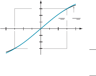
Figure 2 reveals that, even though this partial sum has only two nonzero terms, it is

still a very good approximation to the error function for values of x that are close to

the base point 0.

An Application to

Differential Equations

Equation (8.7.8) tells us that, if we ﬁx a base point, then the power series expansion

of a function, if it has one , is unique Thus if we use one method or formula to

calculate a power series representation f ðxÞ5

n50

ðx 2 cÞ

and if we use a

second method or formula to obtain another power series representation

f ðxÞ5

n50

ðx 2 cÞ

, then a

5 b

for every n (because each is equal to

ðnÞ

ðcÞ=n!). The next example shows how to use this uniqueness to solve a differ-

ential equation.

⁄ EX

AMPLE 8 Find a power series solution of the initial value problem

5 y 2 x; yð0Þ5 2.

Solution Suppos

e that yðxÞ5

n50

. We differentiate term-by-term to obtain

n51

n21

. In order for y to satisfy the given differential equation, we must

have

n51

n21

|ﬄﬄﬄﬄﬄﬄﬄﬄ{zﬄﬄﬄﬄﬄﬄﬄﬄ}

n50

|ﬄﬄﬄﬄﬄ{zﬄﬄﬄﬄﬄ}

2 x:

It is convenient to make the change of summation index m 5 n 2 1 for the series on

the left side. Because n runs from 1 to inﬁnity, the new index m runs from 0 to

inﬁnity. Consequently, we have

m50

ðm 1 1Þa

m11

n50

2 x:

Renaming the index of summation of the series on the left, we obtain

n50

ðn 1 1Þa

n11

n50

2 x:

By separating the terms that correspond to n 5 0 and n 5 1, we may write this

equation as

1 2a

x 1

n52

ðn 1 1Þa

n11

5 a

1 ða

2 1Þx 1

n52

The uniqueness theorem that we discussed allows us to match up coefﬁcients and

deduce that a

5 a

,2a

5 a

2 1, and (n 1 1)

an11

5 a

for n $ 2. The initial condition

y(0) 5 2 tells us that a

5 2. It follows that a

5 2, and a

5 (a

2 1)/2 5 (2 2 1) /2

5 1/2. Substituting n 5 2 in the equation (n 1 1)

an11

5 a

, we obtain a

5 a

/3 5 1/3!.

Substituting n 5 3 in the equation (n 1 1)

an11

5 a

, we obtain a

5 a

/4 5 1/4!. Con-

tinuing in this way, we obtain a

5 1/n! for n $ 2. It follows that, on its interval of

convergence,

0.8

0.6

0.4

0.2

0.4

0.6

0.40.8 0.4

erf(x)



冑

m Figure 2

692 Chapter

8 Inﬁnite Series

yðxÞ5 2 1 2x 1

n52

ð8:7:9Þ

is the solution of the given initial value problem. Because Example 6 of Section 8.6

shows that the power series on the right side of (8.7.9) converges on the entire real

line, we can be sure that equation (8.7.9) provides the complete solution of the given

initial value problem.

Taylor Series and

Polynomials

Theorem 6 of Section 8.7 tells us that, if we hope to represent a function f by a

power series on an open interval I containing c, then f must be inﬁnitely differ-

entiable on I.Iff does have this property, then we may form the power series

TðxÞ5

n50

ðnÞ

ðcÞ

ðx 2 cÞ

: ð8:7:10Þ

We call T(x) the Tay lor series of f with base point c. A Taylor series with base point

0 is also called a Maclaurin series. Theorem 1 of Section 8.7 tells us that T(x) is the

only power series with base point c that can represent f on an open interval cen-

tered at c. Whether it does represent f or not requires analysis. The ﬁrst question is,

does Taylor series (8.7.10) converge at points other than the base point? That

question can be resolved by calculating the radius of convergence in a standard

way. However, even if a Taylor series T(x) generated by a function f has a positive

radius of convergence, it is not automatic that T(x ) is equal to f (x). We will devote

the next section to this question. For now, we will concern ourselves only with the

partial sums of Taylor series.

DEFINITION

If a function f is N times continuously differentiable on an

interval containing c, then

ðxÞ5

n50

ðnÞ

ðcÞ

ðx 2 c Þ

ð0Þ

ðcÞ

ðx 2 cÞ

ð1Þ

ðcÞ

ðx 2 cÞ

ð2Þ

ðcÞ

ðx 2 c Þ

ð3Þ

ðcÞ

ðx 2 cÞ

1 

ðNÞ

ðcÞ

ðx 2 cÞ

is called the Taylor polynomial of order N and base point c for the funct ion f.

THEOREM 2

Suppose that f is N times continuously different iable. Then

ðcÞ5 f ðcÞ; Tu

ðcÞ5 f uðcÞ; Tv

ðcÞ5 f vðcÞ;

ð3Þ

ðcÞ5 f

ð3Þ

ðcÞ;:::T

ðNÞ

ðcÞ5 f

ðNÞ

ðcÞ:

8.7 Representing Functions by Power Series 693

Proof. Fix an integer k between 0 and N. By divi ding T

into three parts,

ðxÞ5

k21

n50

ðnÞ

ðcÞ

ðx 2 cÞ

|ﬄﬄﬄﬄﬄﬄﬄﬄﬄﬄﬄﬄﬄﬄﬄ{zﬄﬄﬄﬄﬄﬄﬄﬄﬄﬄﬄﬄﬄﬄﬄ}

n,k

ðkÞ

ðcÞ

ðx 2 cÞ

|ﬄﬄﬄﬄﬄﬄﬄﬄﬄﬄﬄ{zﬄﬄﬄﬄﬄﬄﬄﬄﬄﬄﬄ}

n5k

n5k11

ðnÞ

ðcÞ

ðx 2 c Þ

|ﬄﬄﬄﬄﬄﬄﬄﬄﬄﬄﬄﬄﬄﬄﬄﬄﬄ{zﬄﬄﬄﬄﬄﬄﬄﬄﬄﬄﬄﬄﬄﬄﬄﬄﬄ}

n.k

;

we see, as in Theor em 1, that

ðxÞ



x5c

5 0 1

ðkÞ

ðcÞ

 k! 1 0 5 f

ðkÞ

ðcÞ:

Thus T

ðkÞ

ðcÞ5 f

ðkÞ

ðcÞ. ’

INSIGHT

Because 0! 5 1, f

(0)

5 1, the ﬁrst term,

ð0Þ

ðcÞ

ðx 2 cÞ

;

of a Taylor polynomial always simpliﬁes to f (c). The longer, unsimpliﬁed, notation serves

to emphasize that the ﬁrst term ﬁts the pattern of all the other terms.

⁄ EXAMPLE 9 Compute the Taylor polynomials of order one, two, and

three for the function f (x) 5 e

expanded with base point c 5 0.

Solution First

of all,

f ð0Þ5 1

ð1Þ

ð0Þ5 2  e

x50

5 2

ð2Þ

ð0Þ5 4  e

x50

5 4

ð3Þ

ð0Þ5 8  e

x50

5 8:

Therefore

ðxÞ5

f ð0Þ

ðx 2 0Þ

ð1Þ

ð0Þ

ðx 2 0Þ

5 1 1 2x;

ðxÞ5

f ð0Þ

ðx 2 0Þ

ð1Þ

ð0Þ

ðx 2 0Þ

ð2Þ

ð0Þ

ðx 2 0Þ

5 1 1 2x 1 2x

and

ðxÞ5

f ð0Þ

ðx 2 0Þ

ð1Þ

ð0Þ

ðx 2 0Þ

ð2Þ

ð0Þ

ðx 2 0Þ

ð3Þ

ð0Þ

ðx 2 0Þ

5 1 1 2x 1 2x

See Figure 3.

INSIGHT

If T

(x) has been computed, then we need not start from scratch in

computing the next Taylor polynomial T

N11

(x); we have only to compute and add one

more term:

N11

ðxÞ5 T

ðxÞ1

ðN11Þ

ðcÞ

ðN 1 1Þ !

ðx 2 cÞ

N11

: ð8:7:11Þ

0.5

0.5

f(x)

(x)

m Figure 3

694 Chapter

8 Inﬁnite Series