Bhushan B. Handbook of Micro/Nano Tribology, Second Edition

Подождите немного. Документ загружается.

building near 100 Hz. This requires a spring with extremely low vertical spring constant (typically, 0.05 to

1 N/m) as well as low mass (on the order of 1 ng). Today, the most-advanced AFM cantilevers are

microfabricated from silicon, silicon dioxide, or silicon nitride using photolithographic techniques. (For

further details on cantilevers, see Section 1.3.2.6.) Typical lateral dimensions are on the order of 100 µm

with the thicknesses on the order of 1 µm. The force on the tip due to its interaction with the sample is

sensed by detecting the deﬂection of the compliant lever with a known spring constant. This lever

deﬂection (displacement smaller than 0.1 nm) has been measured by detecting tunneling current similar

to that used in STM in the pioneering work of Binnig et al. (1986a) and later used by Giessibl et al.

(1991), by capacitance-detection (Neubauer et al., 1990; Goddenhenrich et al., 1990), and by four optical

techniques, namely, (1) by optical interferometry (Mate et al., 1987; McClelland et al., 1987; Erlandsson

et al., 1988a; Mate, 1992; Jarvis et al., 1993) and with the use of optical ﬁbers (Ruger et al., 1989; Albrecht

et al., 1992); (2) by optical polarization detection (Schonenberger and Alvarado, 1990); (3) by laser diode

feedback (Sarid et al., 1988); and (4) by optical (laser) beam deﬂection (Meyer and Amer, 1988, 1990a,b;

Marti et al., 1990). More recently, Smith (1994) used a piezoresistive cantilever beam which requires no

external sensor. It makes the SPM design simpler and the STM and AFM functions can be combined

readily. However, the piezoresistive beam needs power on the order of 10 mW and has less sensitivity.

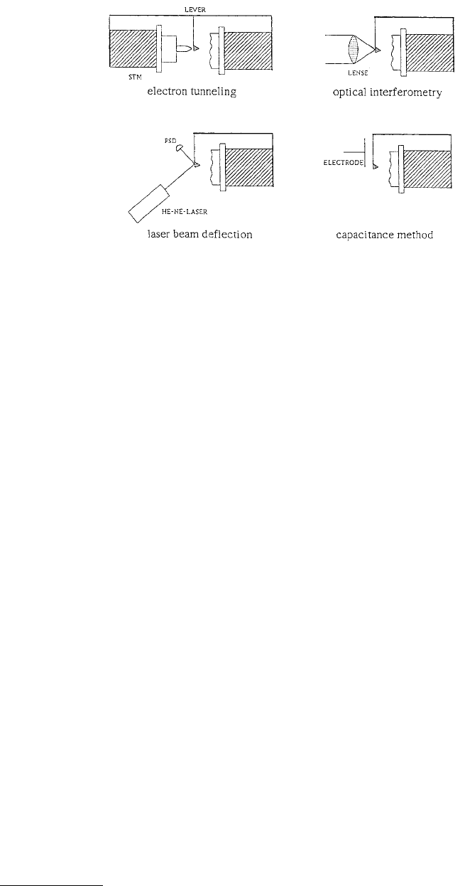
Geometries of the four more commonly used detection systems are shown in Figure 1.12. The tunneling

method originally used by Binnig et al. (1986a) in the ﬁrst version of AFM uses a second tip to monitor

the deﬂection of the cantilever with its force-sensing tip. Tunneling is rather sensitive to contaminants

and the interaction between the tunneling tip and the rear side of the cantilever can become comparable

to the interaction between the tip and sample. Tunneling is rarely used and is mentioned earlier for

historical purposes. Giessibl et al. (1991) recently used it for a low-temperature AFM/STM design. In

contrast to tunneling, other deﬂection sensors are far away from the cantilever at distances of microns

to tens of millimeters. The optical technique is believed to be a more sensitive, reliable, and easily

implemented detection method than others (Sarid and Elings, 1991; Meyer, 1992). The optical beam

deﬂection method has the largest working distance, is insensitive to distance changes, and is capable of

measuring angular changes (friction forces); therefore, it is most commonly used in commercial SPMs.

Almost all AFMs use piezotranslators to scan the sample, or alternatively, to scan the tip. An electric

ﬁeld applied across a piezoelectric material causes a change in the crystal structure, with expansion in

some directions and contraction in others. A net change in volume also occurs (Ashcroft and Mermin,

1976). The ﬁrst STM used a piezotripod for scanning (Binnig et al., 1982). The piezotripod is one way

FIGURE 1.12 Geometries of the four commonly used detection systems for measurement of cantilever deﬂection.

In each setup, the sample mounted on piezoelectric body is shown on the right, the cantilever in the middle, and

the corresponding deﬂection sensor on the left. (From Meyer, E. (1992), Surf. Sci., 41, 3–49. With permission.)

to generate three-dimensional movement of a tip attached to its center. However, the tripod needs to be

fairly large (~50 mm) to get a suitable range. Its size and asymmetric shape makes it susceptible to thermal

drift. The tube scanners are widely used in AFMs (Binnig and Smith, 1986). These provide ample scanning

range within a small size.

Control electronics systems for AFMs can use either analog or digital feedback. Digital feedback circuits

might be better suited for ultralow noise operation.

Images from the AFMs need to be processed. An ideal AFM is a noise-free device that images a sample

with perfect tips of known shape and has perfect linear scanning piezo. In reality, scanning devices are

affected by distortions for which corrections must be made. The distortions can be linear and nonlinear.

Linear distortions mainly result from imperfections in the machining of the piezotranslators causing

cross talk between the Z-piezo to the X- and Y-piezos, and vice versa. Nonlinear distortions mainly result

because of the presence of a hysteresis loop in piezoelectric ceramics. These may also result if the scan

frequency approaches the upper frequency limit of the X- and Y-drive ampliﬁers or the upper frequency

limit of the feedback loop (Z-component). In addition, electronic noise may be present in the system.

The noise is removed by digital ﬁltering in the real space (Park and Quate, 1987) or in the spatial frequency

domain (Fourier space) (Cooley and Turkey, 1965).

Processed data consists of many tens of thousand of points per plane (or data set). The output of the

ﬁrst STM and AFM images were recorded on an X-Y chart recorder, with Z-value plotted against the tip

position in the fast-scan direction. Chart recorders have slow response so storage oscilloscopes or com-

puters are used for display of the data. The data are displayed as wire mesh display or gray scale display

(with at least 64 shades of gray).

1.3.2.1 Binnig et al.’s Design

In the ﬁrst AFM design developed by Binnig et al. (1986a), AFM images were obtained by measurement

of the force on a sharp tip created by the proximity to the surface of the sample mounted on a three-

dimensional piezoelectric scanner. The tunneling current between the STM tip and the backside of the

cantilever beam with attached tip was measured to obtain the normal force. This force was kept at a

constant level with a feedback mechanism. The STM tip was also mounted on a piezoelectric element

to maintain the tunneling current at a constant level.

1.3.2.2 McClelland et al.’s Design

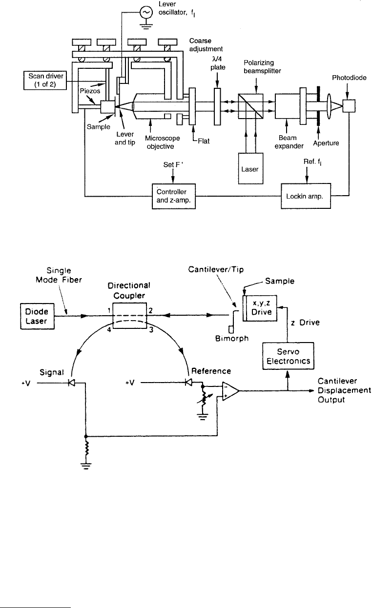
An AFM developed by Erlandsson et al. (1988a) for operation in ambient air is shown schematically in

Figure 1.13. Following the STM design, the test sample was mounted on three orthogonal piezoelectric

tubes (2 to 5 mm long), two of which (x, y) raster the sample in the surface plane while the third (z)

moves the sample toward and away from the tip. The lever was made from a 70-µm-diameter, 3-mm-

long tungsten microprobe with a 90° bend near one end that serves as the tip. (In most cases, the tip is

electrochemically etched using a 12-V AC in 2 N (normal) NaOH solution to obtain a nominal tip radius

between 150 to 300 nm.) The main resonant frequency of this lever was about 5 kHz and the force

constant was about 30 N/m. The lever support was mounted on a piezoelectric transducer that makes it

possible to oscillate the lever when needed. The lever motion was measured by optical interference. A

light beam was focused on the backside of the lever by a microscope objective, and the interference

pattern between the reﬂected beam and a reference beam reﬂected from an optical ﬂat is projected on a

photodiode that measures the instantaneous deﬂection of the lever as well as its vibration amplitude at

high frequencies. The deﬂection can be detected within ±0.2 nm; so for a typical lever force constant of

10 N/m a force as low as 0.2 nN could be detected.

More recently, a high-sensitivity ﬁber-optic displacement sensor has been developed by the IBM group

which is compact and does not require specular reﬂection and thus is compatible with both microfab-

ricated thin-ﬁlm cantilevers as well as ﬁne wire cantilevers. All ﬁber construction results in smaller size

and improved mechanical robustness (Rugar et al., 1989; Albrecht et al., 1992). Schematic design of the

AFM with a ﬁber optic interferometer is shown in Figure 1.14. A multimode GaAlAs diode laser with a

direct single-mode ﬁber output is used as a light source. The light is coupled into the input (labeled “1”)

of a 2 × 2 single-mode directional coupler. The coupler splits the incident optical power equally between

leads 2 and 3, which carry the light to the AFM cantilever and the “reference” photodiode, respectively.

Approximately 4% of the light in lead 2 is reﬂected from the glass–air interface at the cleaved end of the

ﬁber. This reﬂected light comprises one of the two interfering beams. The other 96% of the light exits

the ﬁber and impinges on the cantilever with a spot size of about 5 µm. Part of this light is scattered

back into the ﬁber and interferes with the light reﬂected from the ﬁber end. The total optical power

reﬂected back through the ﬁber depends on the phase difference between the ﬁber end reﬂection and

FIGURE 1.13 Schematic of an AFM which uses optical interference to detect the lever deﬂection. (Erlandsson, R.

et al. (1988), J. Vac. Sci. Technol., A6, 266–270. With permission.)

FIGURE 1.14 Schematic of an AFM with a ﬁber-optic interferometer. (From Rugar, D. et al. (1989), Appl. Phys.

Lett., 55, 2588–2590. With permission.)

the cantilever reﬂection. The coupler directs half of the total reﬂected light to lead 4 and into the signal

2 photodiode where the intensity of the optical interference is measured. To reduce reﬂections from the

ends of leads 3 and 4, the ﬁbers were cleaved at a nonorthogonal angle and an index-matching liquid

was placed between the photodiodes and the ﬁber ends. The output of the signal photodiode can be used

directly as the AFM signal (Rugar et al., 1989).

AFMs can be used to obtain topographic images using repulsive contact forces as well as attractive

electrostatic forces. Several methods have been used to detect the forces (Binnig et al., 1986a; Erlandsson

et al., 1988a). In one force-detection method, the signal corresponding to the force can either be used

as a control parameter for the feedback circuit to generate contours of equal force or be displayed directly

without feedback while pressing the tip onto the sample with an average force larger than the recorded

force variations. In another method, a small AC voltage is applied to the z-tube to induce an oscillation

in the sample and, through the force coupling, to the lever. The resultant oscillation in the photodiode

signal is converted by the lock-in ampliﬁer to a voltage that is proportional to the derivative of the force,

F′. The z-ampliﬁer compares the voltage to some preset value and drives the z-tube to form a feedback

loop to maintain F′ constant, and a three-dimensional surface of F′ can be obtained (Erlandsson et al.,

1988a).

1.3.2.3 Kaneko et al.’s Design

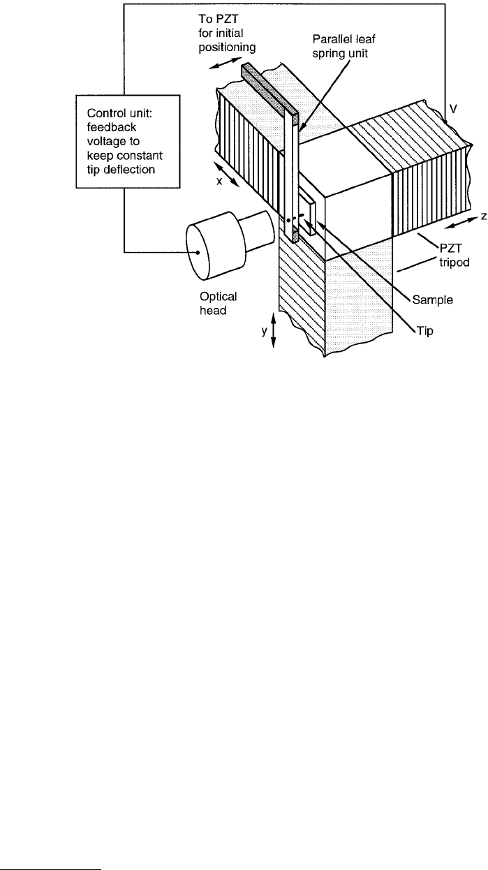
In the AFM designs developed by Kaneko and co-workers for use in ambient air, the instrument consists

of a piezoelectric tripod that holds the sample, a sharp diamond tip (to be presented later) supported

by a parallel-leaf spring unit mounted on a laminated piezoelectric stack, and a focusing error detection

type optical head, Figure 1.15 (Kaneko et al., 1988; Kaneko and Hamada, 1990; Miyamoto et al., 1990).

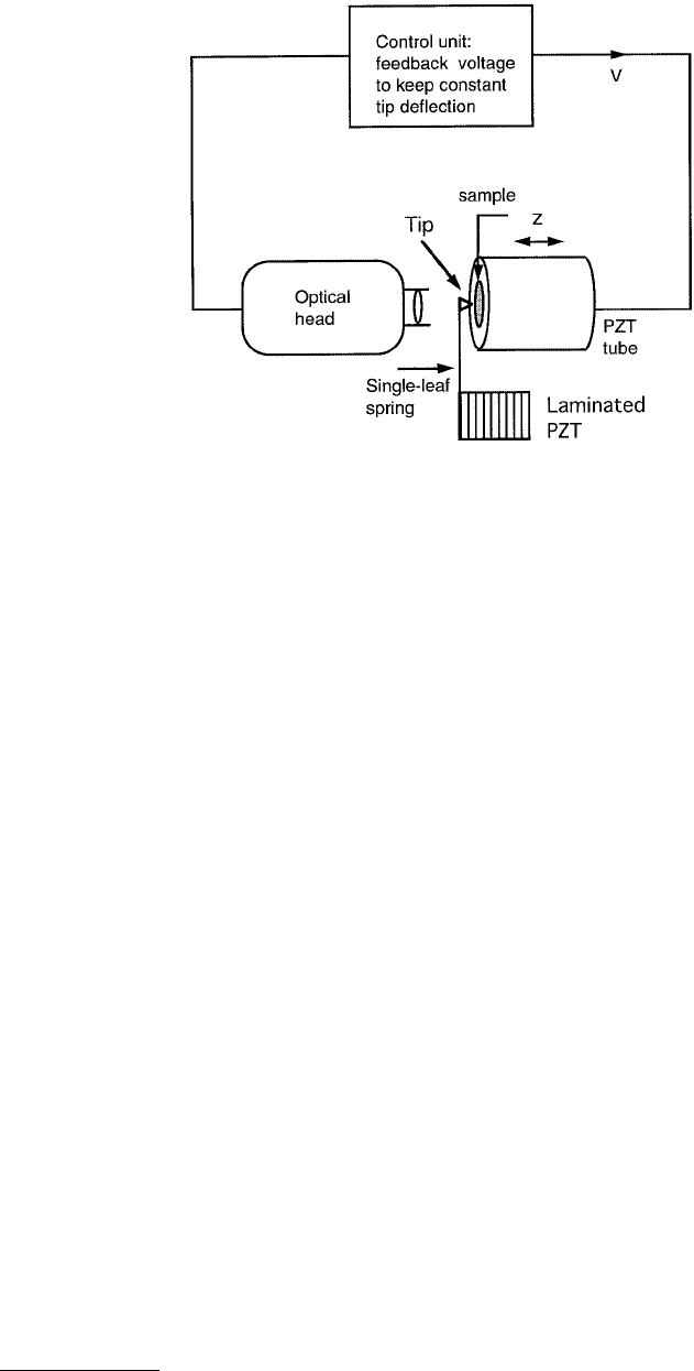
This design was later modiﬁed by Kaneko et al. (1990, 1991). The major modiﬁcations were that a

piezotube scanner was used to hold the sample and the tip was supported on a single-leaf spring,

Figure 1.16. In their even newer design, they have incorporated a new tube scanner and an optical

FIGURE 1.15 Schematic of an AFM in which the sample is mounted on a piezoelectric tripod and the tip is

supported by a parallel-leaf spring unit. (From Kaneko, R. et al. (1988), J. Vac. Sci. Technol., A6, 291–292. With

permission.)

multifunction sensor (Kaneko et al., 1992). The spring constants used in Figures 1.15 and 1.16 are 3 to

24 N/m and 0.3 to 3 N/m, respectively. A laminated piezoelectric stack was used for initial positioning

of the tip and the piezoelectric tripod or piezotube scanner was used to place the tip in contact with the

surface in the z-direction and to scan the surface in the x- or y-direction. For surface topography

measurements, the sample was slowly moved in the z-direction until it contacted the tip then it was

scanned in the x- or y-direction. Tip displacement during scanning was measured by a focusing error-

detection-type optical head (with an accuracy of better than 1 nm), and the displacement signal was

used as a control signal for the z-displacement of the piezoelectric tripold or tube scanner to keep the

spring load constant. Variations in the vertical motion of the sample represented a roughness proﬁle.

Additional details of the construction of these designs can be found in a following FFM section.

1.3.2.4 Meyer and Amer’s Design

In the AFM design developed by Meyer and Amer (1988) for operation in an ultrahigh vacuum (UHV),

bending of a tungsten cantilever beam resulting from the normal force being applied at the tip was

measured by detecting the deﬂection of a laser beam, which was reﬂected off its backside. The deﬂection

was sensed with a segmented photodiode detector, typically a bicell, which consists of two photoactive

(e.g., Si) segments (anodes) that are separated by about 10 µm and have a common cathode. This optical

beam deﬂection technique is simple and sensitive and is used in a commercial AFM whose description

follows.

1.3.2.5 Commercial AFMs

There are a number of commercial AFMs available on the market since 1989. Major manufacturers of

AFMs for use in an ambient environment are Digital Instruments, Inc., 112 Robin Hill Road, Santa

Barbara, CA; Park Scientiﬁc Instruments, 476 Ellis Street, Mountain View, CA; Topometrix, 5403 Betsy

Ross Drive, Santa Clara, CA; Seiko Instruments, Japan; Olympus, Japan; and Centre Suisse D’Electronique

et de Microtechnique (CSEM) S.A., Neuchâtel, Switzerland. In the CSEM design, both force sensors

(using optical beam deﬂection method) and scanning unit are mounted on the microscope head; thus

their AFM/FFM designs can be used as stand-alone (Hipp et al., 1992). UHV AFM/STMs are manufac-

tured by Omicron Vakuumphysik GmbH, Idsteiner Strasse 78, D-6204, Taunusstein 4, Germany. Personal

FIGURE 1.16 Schematic of an AFM in which the sample is mounted on a piezoelectric tube scanner and the tip

is supported by a single-leaf spring. (From Kaneko, R. et al. (1990), Tribology and Mechanics of Magnetic Storage

Systems (B. Bhushan, ed.) SP-29, pp. 31–34, STLE, Park Ridge, IL. With permission.)

STMs and AFMs for ambient environment and UHV/STMs are manufactured by Burleigh Instruments,

Inc., Burleigh Park, Fishers, NY.

We describe here the commercial AFM for operation in ambient air, produced by Digital Instruments,

Inc., with scanning lengths ranging from about 0.7 µm (for atomic resolution) to about 125 µm (Alex-

ander et al., 1989; Anonymous, 1992b; Bhushan and Ruan, 1994a; Ruan and Bhushan, 1994a,b). This is

the most commonly used design and the multimode AFM comes with many capabilities. The original

design of this AFM version comes from Meyer and Amer (1988). Basically, the AFM scans the sample in

a raster pattern while outputting the cantilever deﬂection error signal to the control station. The cantilever

deﬂection (or the force) is measured using a laser deﬂection technique, Figure 1.17. The digital signal

processor (DSP) in the workstation controls the Z-position of the piezo based on the cantilever deﬂection

error signal. The AFM operates in both the constant-height and constant-force modes. The DSP always

adjusts the height of the sample under the tip based on the cantilever deﬂection error signal, but if the

feedback gains are low the piezo remains at a nearly constant height and the cantilever deﬂection data

is collected. With the gains high, the piezo height changes to keep the cantilever deﬂection nearly constant

(therefore, the force is constant), and the change in piezo height is collected by the system. The following

description of the instrument is almost exclusively based on Anonymous (1992b).

To further describe the principle of operation of the commercial AFM, the sample is mounted on a

piezoelectric tube scanner which consists of separate electrodes to scan the sample precisely in the X–Y

plane in a raster pattern as shown in Figure 1.18 and to move the sample in the vertical (Z) direction.

A sharp tip at the free end of a microfabricated ﬂexible cantilever is brought in contact with the sample.

Features on the sample surface cause the cantilever to deﬂect in the vertical direction as the sample moves

FIGURE 1.17 Principle of operation of a commercial AFM/FFM — sample mounted on a piezoelectric tube scanner

is scanned against a sharp tip and the cantilever deﬂection is measured using a laser deﬂection technique.

under the tip. A laser beam generated from a diode laser (light-emitting diodes or LEDs with a 5-mW

max peak output at 670 nm) is directed by a prism onto the back of the cantilever near its free end, tilted

downward at about 10° with respect to a horizontal plane. The reﬂected beam from the vertex of the

cantilever is directed through a mirror onto a quad photodetector (split photodiode detector with four

quadrants commonly called position-sensitive detector or PSD), produced by Silicon Detector Corpora-

tion, 1240 Avenida Acasco, Camarillo, CA. The differential signal from the top and bottom photodiodes

[(T – B)/(T + B)] provides the AFM signal which is a sensitive measure of the cantilever vertical deﬂection.

In the AFM operating mode, the “height mode,” this AFM signal is used as the feedback signal to control

the vertical position of the piezotube scanner and the sample, such that the cantilever vertical deﬂection

(hence the normal force at the tip–sample interface) will remain (almost) constant as the sample is

scanned. Thus, the vertical motion of the tube scanner relates directly to the topography of the sample

surface. We note that normal force and vertical motion of the sample can be independently measured

by the photodiode and the piezoelectric scanner, respectively. Topographic measurements are made using

the height mode at any scanning angle. At a ﬁrst instance, the scanning angle may not appear to be an

important parameter. However, the friction force between the tip and the sample (which we will discuss

later in the FFM section) will affect the topographic measurements in a parallel scan (scanning along

the long axis of the cantilever), therefore, a perpendicular scan may be more desirable. Generally, one

picks a scanning angle which gives the same topographic data in both directions; this angle may be

slightly different than that for the perpendicular scan.

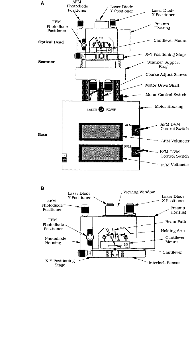
Physically, the AFM consists of three main parts: the optical head which senses the cantilever deﬂection,

a piezoelectric tube scanner which controls the scanning motion of the sample mounted on its one end,

and the base which supports the scanner and head and includes circuits for the deﬂection signal. The

AFM connects directly to a control system. A front view of the AFM is shown in Figure 1.19A. Due to

the weight of the optical head, the sensing system cannot be mounted on the piezo tube, therefore, the

optical head and the cantilever are held stationary while the sample is scanned under them. The optical

sensing system is packaged into the optical head of the microscope (Figure 1.19B). The head consists of

a laser diode stage, a photodiode stage preamp board, a cantilever mount and its holding arm, and a

deﬂection beam reﬂecting mirror. The laser diode stage is a tilt stage used to adjust the position of the

laser beam relative to the cantilever. It consists of the laser diode, collimator, focusing lens, base plate,

and the X and Y laser diode positioners. The positioners are used to place the laser spot on the end of

the cantilever. The photodiode stage is an adjustable stage used to position the photodiode elements

relative to the reﬂected laser beam. It consists of the split photodiode, the base plate, and the photodiode

positioners. The top (AFM) positioner is used to adjust the AFM signal by moving the photodiode up

and down. Similarly, the front (FFM) positioner adjusts the FFM signal by moving the photodiode

elements in and out (used for FFM, to be described later). The preamp board contains preampliﬁer

circuits for all four photodetecter signals and a laser diode power supply circuit. The cantilever mount

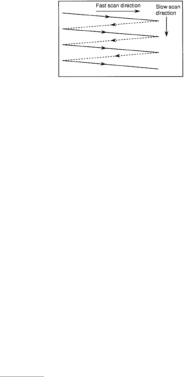
FIGURE 1.18 Schematic of triangular pattern trajectory of the AFM tip as the sample is scanned in two dimensions.

During imaging, data are recorded only during scans along the solid scan lines whereas scratch and wear (to be

described later) take place along both the solid and dotted lines.

is a metal (for operation in air) or glass (for water) block which holds the cantilever ﬁrmly at the proper

angle, Figure 1.19D, and the deﬂection beam reﬂecting mirror is mounted on the upper left in the interior

of the head which reﬂects the deﬂected beam toward the photodiode.

The scanner consists of an Invar cylinder holding a single tube made of piezoelectric crystal which

provides the necessary three-dimensional motion to the sample, Figure 1.6B. Mounted on top of the tube

is a magnetic cap on which the steel sample puck is placed. The tube is rigidly held at one end with the

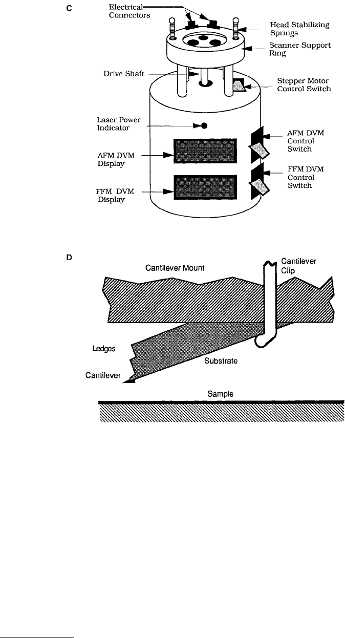
FIGURE 1.19 Schematics of a commercial AFM/FFM made by Digital Instruments, Inc.: (A) front view, (B) optical

head, (C) base, and (D) cantilever substrate mounted on cantilever mount (not to scale). (From “Nanoscope III

Atomic Force Microscope, Instruction Manual,” Courtesy of Digital Instruments, Inc., Santa Barbara, CA., 1992)

sample mounted on the other end of the tube. Samples up to about 10 × 10 mm or about 15 mm in

diameter and 10 mm in thickness can be used. The scanner also contains three ﬁne-pitched screws which

form the mount for the optical head. The optical head rests on the tips of the screws which are used to

adjust the position of the head relative to the sample. The scanner ﬁts into the scanner support ring

mounted on the base of the microscope, Figure 1.19C. Two of the screws on the scanner are operated

manually while the third is controlled with a stepper motor built into the base of the microscope. The

stepper motor is controlled manually with the switch on the upper surface of the base and automatically

by the computer during the tip-engage and tip-withdraw processes. The base also houses electronic

circuits which are essential to the alignment and operation of the microscope. The two liquid-crystal

(digital voltmeter or DVM) displays on the base show either the sum of the photodiode signals or the

differential photodiode signals depending on the position of the respective control switches on the base.

These voltages are required during the optical alignment of the system.

FIGURE 1.19 (continued)

The scan sizes available for this instrument are 0.7, 12, and 125 µm. The scan rate must be decreased

as the scan size is increased. A maximum scan rate of 122 Hz can be used. Scan rates of about 60 Hz

should be used for small scan lengths (0.7 µm). Scan rates of 0.5 to 2.5 Hz should be used for large scans

on samples with tall features. High scan rates help reduce drift, but they can only be used on ﬂat samples

with small scan sizes. Scan rate or scanning speed in length/time is equal to twice the scan length times

the scan rate in Hz, and in the slow direction, it is equal to scan length times the scan rate in Hz divided

by the number of data points in the transverse direction. For example, for 10 × 10 µm scan size scanned

at 0.5 Hz, the scan rates in the fast and slow scan directions are 10 µm/s and 20 nm/s, respectively.

Normally 256 × 256 data points are taken for each image. The lateral resolution at larger scans is

approximately equal to scan length divided by 256. The piezotube requires X–Y calibration which is

carried out by imaging an appropriate calibration standard. Cleaved graphite is used for small scan heads

while two-dimensional grids (a gold-plating ruling) can be used for longer-range heads.

To prepare AFM for imaging, the following steps are required: installing a cantilever, loading a sample,

aligning the optics, and doing the coarse approach of the tip to the sample. By loosening the cantilever

holding-arm screw located on the back of the optical head, the cantilever mount is removed. The

appropriate cantilever is mounted on the cantilever mount with a clip (Figure 1.19D), and the cantilever

mount is replaced into the optical head. The AFM is provided with 12.7-mm-diameter steel pucks that

can be attached to the magnetic cap on the end of the scanner tube. The sample is placed on the puck

by using a sticky tab or a quick-drying glue and the puck is placed onto the magnetic cap on the top of

the scanner tube. Next, the optical head is placed on the magnetic balls mounted on the ends of the three

screws of a scanner on which the sample has already been loaded. When the head is in place, electrical

connections are made. Next the laser, cantilever, and photodiode are aligned. While observing the

substrate/cantilever through a magniﬁer, the laser spot is adjusted with the two positioning knobs on

the top of the head so that it is positioned on the vertex of the cantilever. After the laser beam is properly

aligned with the cantilever, photodiode positioners are adjusted to center the laser spot in the quad

photodiode. As a ﬁrst step, the laser spot is centered visually then centered more precisely to maximize

the AFM sum signal (T + B), while setting the FFM difference signal (L – R) to zero (for friction

measurements, to be discussed later). When the AFM sum signal is maximized, one should see a signal

of 5 to 9 V. After optical alignment, the cantilever is lowered with the coarse-approach screw until the

tip is about 0.1 mm above the sample, followed by the ﬁne position of the tip by monitoring the reﬂection

of the illuminated cantilever on the sample (tip must not touch the sample). A ﬁnal step prior to engaging

is the setting of the AFM control switch to difference signal (down position) and the adjustment of the

photodiode position until the output of the preamp is set to a desirable value, between –1 and –4 V.

Now the AFM is ready for scanning, which is initiated by engaging the microscope.

Examples of AFM images of freshly cleaved HOP graphite and mica surfaces are shown in Figure 1.20

(Albrecht and Quate, 1987; Marti et al., 1987; Ruan and Bhushan, 1994b).

Force calibration mode is used to study interaction between the cantilever and the sample surface. In

the force calibration mode, the X- and Y-voltages applied to the piezotube are held at zero and a sawtooth

voltage is applied to the Z-electrode of the piezotube, Figure 1.21A. The force measurement starts with

the sample far away and the cantilever in its rest position. As a result of the applied voltage, the sample

is moved up and down relative to the stationary cantilever tip. As the piezo moves the sample up and

down, the cantilever deﬂection signal from the photodiode is monitored. The force curve, a plot of the

cantilever deﬂection signal as a function of the voltage applied to the piezotube, is obtained. Figure 1.21B

depicts a typical force–separation curve showing the various features of the curve. The arrow heads reveal

the direction of piezo travel. At point 1, the tip is off the sample surface. From point 1 to point 2 there

is no change in the deﬂection signal as the piezo extends, because the force is initially zero as the sample

has not come into contact with the tip. At point 2 the tip is a fraction of a nanometer away from the

sample, and the force between the tip and the sample suddenly becomes attractive. The cantilever bends

toward the sample and the attractive force increases gradually until point 2′ of the sample and tip come

into intimate contact and the force becomes repulsive. The maximum forward deﬂection of the cantilever