Barber J.R. Intermediate Mechanics of Materials

Подождите немного. Документ загружается.

4.4 Further properties of second moments 215

′

= −1.66 cos(37.2

) −(−0.657)sin(37.2

) = −0.93 in.

Substituting these values in the equation for

, we then have

= 279.5(3.06) + 1422(1.50) = 2983 psi (maximum tensile stress)

and

= 279.5(−0.93) + 1422(−1.53) = −2436 psi (maximum compressive stress) .

4.4.4 Design estimates for the behaviour of unsymmetrical sections

Arguably, the greatest practical use of the coordinate transformation relations and

Mohr’s circle of second moments of area is to enable us to draw general conclusions

that provide insight into the behaviour of unsymmetrical beam sections. We have

already remarked on some of these properties in §4.4.2 and in this section we shall

show how related arguments can be developed to permit quite accurate estimates to

be made for the location of the principal axes and the neutral axis of bending, without

doing any calculations.

We showed in §4.3.2 that out of the class of all axes parallel to a given direction,

that through the centroid has the lowest value of

I =

dA , (4.53)

where n is the perpendicular distance from a given elemental area dA to the axis.

The Mohr’s circle results show that if we now change the direction of the axis, the

lowest value of I corresponds to the ﬂexible principal axis 2 in Figure 4.21. Thus,

the ﬂexible centroidal principal axis corresponds to the absolute minimum value of

I for axes of all inclinations and positions and we could reformulate the question of

determining it as a minimization problem — i.e. determine the axis for which I as

deﬁned by equation (4.53) is a minimum.

Now recall that the usual procedure for ﬁnding the ‘best’ straight line approxima-

tion to a set of experimental points is to choose that line which minimizes the sum of

the squares of the distances n

of the individual points from the line — i.e. minimize

|E|

≡

∑

i=1

. (4.54)

This is known as the ‘least squares ﬁt’ and it is exactly similar to the minimization

of (4.53) except that in the latter case we have elemental areas dA instead of points.

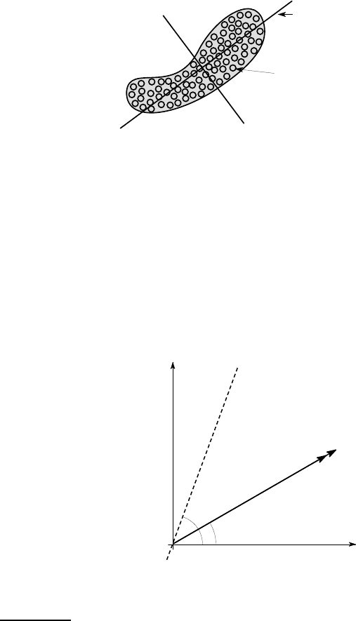
Thus, if we imagine dividing up the section into equal small areas and place one

imaginary point at the centre of each, the ﬂexible axis will be the best straight line

ﬁt to the resulting set of points. We can ﬁnd this line quite well by eye, as shown in

216 4 Unsymmetrical Bending

Figure 4.27, provided the section is reasonably ‘long and thin’ — which is equiv-

alent to the statement that the maximum and minimum second moments should be

signiﬁcantly different.

"best fit"

flexible axis

stiff axis

imaginary

experimental

points

Figure 4.27: Estimating the principal axes using the ‘least squares ﬁt’ method

Once we have estimated our best straight line — corresponding to the ﬂexible

axis — the stiff axis can be found by estimating the location of the centroid (which

must lie on the ﬂexible axis) and then drawing a line through it at right angles to the

ﬂexible axis as shown.

Location of the neutral axis

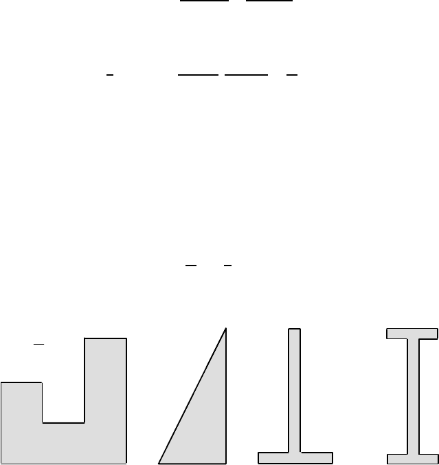
We shall now show that the neutral axis will always lie between (i) the ﬂexible prin-

cipal axis and (ii) the axis about which the bending moment is applied (see Figure

4.28). The bigger the ratio between I

and I

, the closer the neutral axis will get to

the ﬂexible axis.

neutral

axis

1 (stiff)

2 (flexible)

Figure 4.28: Location of the neutral axis

If they are not, it doesn’t matter too much from an engineering perspective where the prin-

cipal axes are anyway, since the maximum product inertia is (I

−I

)/2, from Figure 4.21

and hence the coupling effect will be weak — i.e. the elementary theory will give quite

good answers.

4.4 Further properties of second moments 217

To demonstrate this, we ﬁrst resolve the applied moment M into components

about the principal axes — i.e.

= M cos

; M

= M sin

. (4.55)

Substitution into (4.52) then gives

My cos

−

Mx sin

(4.56)

and the neutral axis (

=0) is deﬁned by the equation

= tan

M sin

M cos

tan

. (4.57)

Since I

by deﬁnition, it follows that |tan

|>|tan

|and hence that |

|>|

Furthermore, |tan

| increases with the ratio I

(i.e. the neutral axis moves closer

to the ﬂexible axis) for all

except

= 0. In particular, a section with a very large

ratio I

will tend to bend about the ﬂexible axis, regardless of the direction of the

applied moment. You can test this experimentally with a thin plastic ruler.

These results provide a convenient method of estimating the location of the neu-

tral axis and hence the maximum stress points without doing any algebraic calcula-

tions, provided we can estimate the value of the ratio I

. For a rectangular section

a×b, with a >b, this ratio is





, (4.58)

so a plausible ﬁrst estimate is to use the square of the ratio of maximum to minimum

dimensions.

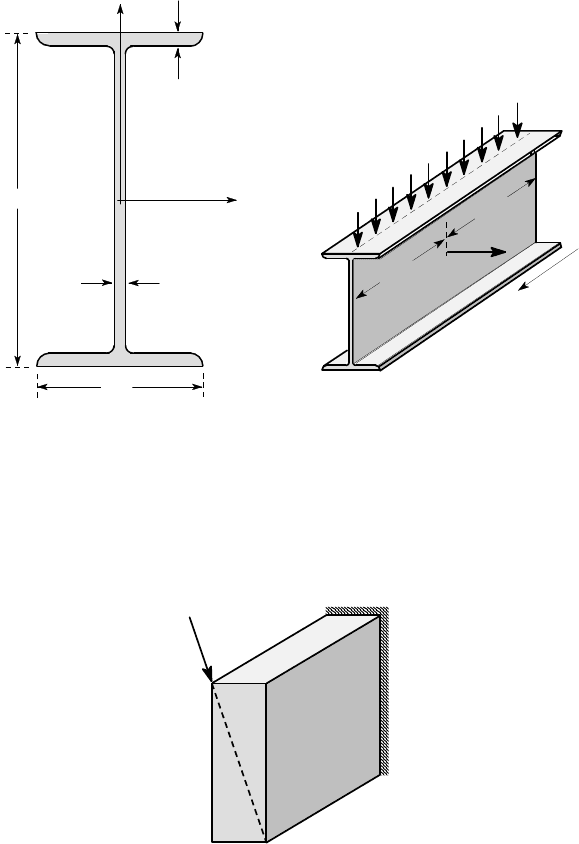
= 2

(a) (b) (c) (d)

Figure 4.29: Values of the ratio I

for some representative beam sections

Figure 4.29 shows a variety of beam sections and the corresponding values of

. Most people are initially surprised that these values are so high, particularly

for sections like Figure 4.29 (a) that appear not too far from equi-axed. However, it

is fairly easy to develop the ability to get a rough estimate at sight and this coupled

with a visual ‘least squares’ estimate of the direction of the ﬂexible axis permits us

218 4 Unsymmetrical Bending

to place the neutral axis with some conﬁdence. It is a good idea to do this as an

initial step even when a full algebraic solution is intended, since the visual estimate

provides a check against algebraic errors. You will be surprised to see how close your

estimate is to the calculated value.

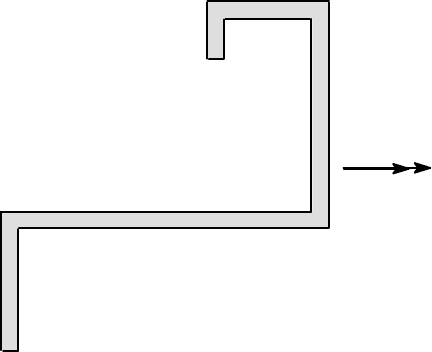
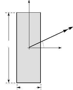
Example 4. 8

The beam section in Figure 4.30 is loaded by a bending moment M about the hor-

izontal axis, as shown. Without doing any calculations, estimate the location of the

principal axes of the section and the resulting neutral axis. Hence identify the points

of maximum tensile and compressive stress in the section.

Figure 4.30

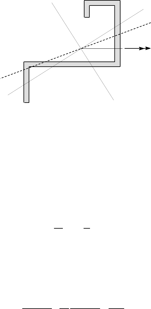
We ﬁrst use the ‘least squares’ argument to estimate the ﬂexible axis 2, as shown

in Figure 4.31. We then estimate the location of the centroid C (which must lie on

the ﬂexible axis) and hence draw in the stiff axis 1, at right angles to 2.

For this section, we estimate the ratio I

≈7, by comparison with the examples

in Figure 4.29. Equation (4.57) therefore implies a fairly substantial movement of the

neutral axis towards the ﬂexible axis which we estimate as shown. (If you like, you

can do a one line calculation using equation (4.57) to estimate

, but you still have

to estimate where this is on the diagram, which we are not drawing strictly to scale,

so probably a guess is good enough here.)

Finally, the maximum tensile and compressive stresses will occur at the points

furthest from the neutral axis — i.e. at A,B in Figure 4.31. To determine which is

which, imagine that the moment arrow is rotated to line up with the neutral axis. A

clockwise moment about this arrow will involve motion out of the paper) at A and

into the paper at B, so the maximum tensile stress will be at A and the maximum

compressive stress at B.

4.4 Further properties of second moments 219

neutral

axis

Figure 4.31

4.4.5 Errors due to misalignment

We have seen that that differences between the two principal second moments cause

the neutral axis to deviate considerably from the moment axis towards the direction

of the ﬂexible principal axis. This effect can be particularly important if the section

is designed to have a large value of I

about the axis where bending is anticipated,

since small variations in the moment axis, due perhaps to misaligment of supports or

loading, can then cause signiﬁcant increase in stresses and deﬂections.

As an example, we consider a rectangular section of aspect ratio 10, subjected to

a moment M

, whose axis deviates from the stiff axis by the small angle 0.01 radians

(= 0.6

), as shown in Figure 4.32 (a). Notice that the angle actually drawn in this

ﬁgure is exaggerated by a factor of 10 for clarity.

The two principal second moments are

; I

, (4.59)

so that the ratio I

= 100.

The neutral axis is therefore deﬁned by

tan

= 100 tan(0.01) ≈1 ,

from equation (4.57). Thus, the beam bends about an axis inclined at 45

to the stiff

axis, despite the fact that the moment is only very slightly misaligned (see Figure

4.32 (b)).

We also calculate the maximum tensile stress, which will occur at A. We have

×5 ×12

1000

−

100

(−0.5) ×12

6.6M

100

, (4.60)

from (4.52).

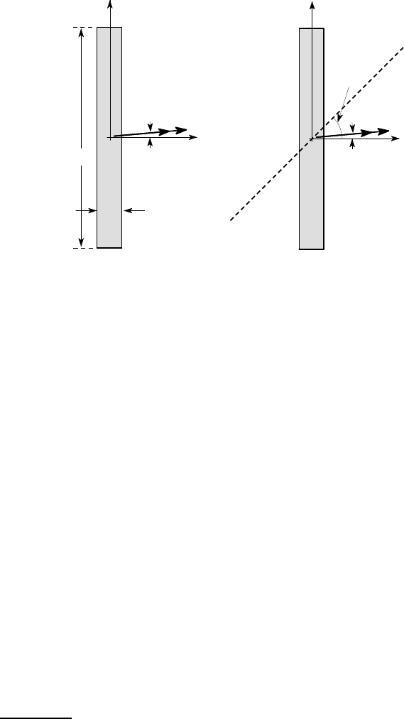
220 4 Unsymmetrical Bending

0.01 rad.

neutral

axis

(a) (b)

Figure 4.32: Effect of moment misalignment

Without the misalignment, the result would be 6M

/100, so the error is only 10%

which is not too serious. However, the unwanted out of plane ﬂexure of the beam

could be a problem. For beams with a larger ratio between I

and I

, misalignment

could have more serious effects. This effectively places a limit on the extent to which

beams can be tailored to give high strength and stiffness about a speciﬁed moment

axis.

4.5 Summary

In this chapter, we have extended the elementary theory of elastic bending to beams

of arbitrary cross section. All sections posess an orthogonal pair of principal axes

which are respectively the stiffest and the most ﬂexible axes for bending. The ele-

mentary theory of bending is exact when the bending moment is applied about one of

the principal axes, but in all other cases it is non-conservative — the actual stresses

will be larger than those predicted by the elementary theory and the errors can be

quite large. These errors stem from the fact that the axis of bending (the neutral axis)

generally deviates from the moment axis in unsymmetrical beams.

The engineering designer should pay particular attention to §4.4.4, in which

methods are discussed for estimating the location of the principal axes of a section

and the neutral axis of bending by eye. These methods enable us to judge when the

deviation of the neutral axis (and hence the errors in the elementary bending predic-

tion) will be large enough to warrant the extra complexity of a full unsymmetrical

bending calculation. Situations where this happens are generally undesirable,

since

Ask yourself why you are proposing to use an unsymmetrical section in bending. Legiti-

mate reasons include the convenience of attachment of devices to the beam or geometrical

constraints on the volume which it occupies.

Problems 221

they imply that signiﬁcant bending is occurring about the ﬂexible (and hence weaker)

axis.

The stiffness of a beam in bending is governed by the second moments of area

of the section. Methods have been presented for determining the second moments

in a speciﬁc coordinate system. Mohr’s circle can be used to transform these results

to other axis systems and, in particular, to determine the principal values and the

inclination of the principal axes.

Unsymmetrical bending effects are most pronounced when the ratio of princi-

pal second moments (I

) is large. Such beams may appear to be optimal when

bending moments are expected only about one axis, but they are very sensitive to

manufacturing or assembly imperfections or load misalignment.

Further reading

W.B. Bickford (1998), Advanced Mechanics of Materials, Addison Wesley, Menlo

Park, CA, pp. 182–204.

A.P. Boresi, R.J. Schmidt, and O.M. Sidebottom (1993), Advanced Mechanics of

Materials, John Wiley, New York, 5th edn., Chapter 7.

Problems

Section 4.1.4

4.1. Figure P4.1 shows the cross section of a rectangular beam which is subjected

to a bending moment of 500 Nm inclined at 25

to the x-axis. Find the location and

magnitude of the maximum tensile stress due to bending.

500 Nm

20 mm

60 mm

Figure P4.1

222 4 Unsymmetrical Bending

4.2. Figure P4.2 shows the dimensions of a W200×22 I-beam, for which I

=20×10

, I

=1.42×10

. The length of the beam is 10 m and it is simply supported

at its ends. The loading consists of a downward vertical distributed load of 1000 N/m

throughout the length of the beam (i.e. in the negative y-direction) and a horizontal

concentrated force of 1000 N in the positive x-direction located at the mid-point

of the beam. Find the magnitude and location of the maximum tensile stress in the

beam.

102

6.2

206

O x

5 m

1000 N/m

1000 N

all dimensions in mm.

Figure P4.2

4.3. A cantilever beam of rectangular cross section is loaded by a force F directed

along the diagonal AC of the section as shown in Figure P4.3. Show that the neutral

axis in this case coincides with the other diagonal BD for all values of the dimensions

a,b of the rectangle.

Figure P4.3

Problems 223

4.4. A beam of rectangular cross section (a×b) is loaded by a compressive axial

force F whose line of action passes through the point (c,d) in centroidal coordinates

Oxy. Find the range of values of c,d for which the stress at all points in the section

remains compressive.

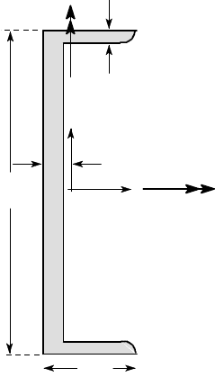
4.5. The C200×20 channel section of Figure P4.5 has second moments of area I

15×10

, I

=0.637×10

. It is loaded by the bending moments M

=2200

Nm and M

= −350 Nm. Find the magnitude and location of the maximum tensile

stress in the beam.

-350 Nm

15.6

2200 Nm

203

59.5

9.9

all dimensions in mm.

Figure P4.5

Section 4.1.5

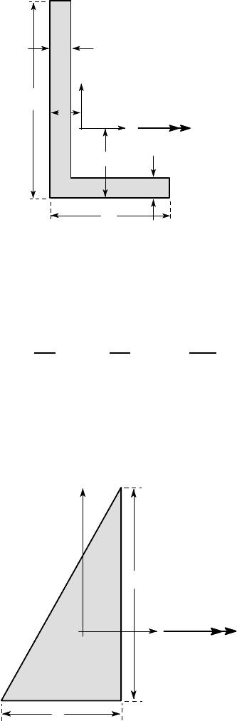
4.6. The L-section shown in Figure P4.6 has second moments I

= 1,512,500

, I

= 412, 500 mm

, I

= −450,000 mm

about centroidal axes Oxy. The cen-

troid is located at the point (15,35) relative to the corner C as shown.

The beam is subjected to a bending moment M = 1000 Nm about the horizontal

axis Ox. Find the inclination of the neutral axis to Ox and the location and magnitude

of the maximum tensile stress in the section.

Compare your results with the value My

max

from the elementary bending the-

ory.

224 4 Unsymmetrical Bending

1000 Nm

100

all dimensions in mm.

Figure P4.6

4.7. The second moments of area for the right-angle triangular section of Figure P4.7

are

; I

and the centroid O is located a distance a/3 above and b/3 to the left of B.

A beam of this section is loaded by a bending moment M

about the x-axis —

i.e. M

, M

=0. Show that the neutral axis is deﬁned by the line joining C to the

mid-point of AB.

Comment on the implications of this result when b≪a.

Figure P4.7