Appel W. Mathematics for Physics and Physicists

Physical applications, the C auchy problem 347

12.5.b A simple example

The Laplace transform can be used to s olve a differential equation, taking

initial conditions into account, in a more natural manner than wit h the

Fourier transform.

The b est is to start with a simple example. Suppose we want to solve the

following Cauchy problem:

(C )



¨x + x = 2 cos t,

x(0) = 0 ˙x(0) = −1.

We a ssume that the function x has a Laplace transform: x(t) ⊐ X (p). Then

the second derivative of x has the following Laplace transform, which incor-

porates the initial conditions:

¨x(t) ⊐ p

X (p) − p x(0) − ˙x(0) = p

X (p) + 1,

while

cos t ⊐

+ 1

The differential equation (with the given initial conditions) can therefore be

written simply in the form

X (p) + 1 + X (p) =

+ 1

which is solved, in th e sense of functions

, by putting

X (p) =

+ 1)

−

+ 1

There only remains to ﬁnd the original of X (p). The second term on the

right-hand side of the preceeding relation is the image of the sine function:

sin t ⊐ 1/(p

+ 1). Moreover, using Theorem 12.21, we obtain

t sin t ⊐ −



+ 1



+ 1)

which gives the solution X (p) ⊏ t sin t −sin t = (t − 1) sin t.

It is easy to check that x(t) = (t −1) sin t is indeed a solution of the stated

Cauchy problem.

The reader is referred to the table on page 614 for a list of the principal

Laplace transforms.

One can see the advantage of working wit h Laplace transforms, which are functions,

instead of Fourier transforms, which are distributions.

348 The Laplace transform

12.5.c D ynamics of the electromagnetic ﬁeld w ithout sources

The example treated here is somewhat more involved.

Consider the free e volution of th e electromagnetic ﬁeld in the space R

, in

the absence of a ny source. For reasons of simplicity, it is easier to study the

evolution of the potential four-vector A( r, t) in Lorenz gauge instead of the

evolution of the electric and magnetic ﬁelds. The initial conditions at t = 0

are given by the data of the ﬁeld A( r, 0) = A

( r) and of its ﬁrst derivative

with respect to t ime, which we denote by

( r).

The equations which determine the ﬁeld are therefore







A( r, t) = 0 for all r ∈ R

and t > 0,

A( r, 0) = A

( r) for all r ∈ R

A( r, 0) =

( r) for all r ∈ R

We denote by AA

AA ( r, p) the Laplace transform of A( r, t), and by

A(k, t) its

Fourier transform with respect to the space variable. We also denote by

AA ( k, p) the double transform (Laplace transform for the variable t and

Fourier transform for the variable r).

We have, by the differentiation theorem 12.19 :

A( r, t) ⊐ AA

AA ( r, p),

∂

∂ t

A( r, t) ⊐ pAA

AA ( r, p) −A( r, 0),

∂

∂ t

A( r, t) ⊐ p

AA ( r, p) − pA( r, 0) −

A( r, 0),

and the evolution of the potential is therefore described, in the Laplace world,

by the equation



−△



AA ( r, p) =

( r) +

( r).

Take then the Fourier transform for the space var iable, which gives



+ k



AA ( k, p) =

(k) +

(k),

AA ( k, p) =

+ k

(k) +

+ k

(k),

from which we can now take the inverse Laplace transform to derive, for any

t ¾ 0, th at

A(k, t) =

(k) H (t) cos(kc t) +

(k)

H (t) sin(kc t)

Finally we need only compute the inverse Fourier of t 7→ (sin kc t)/kc and

t 7→ cos(kc t).

Physical applications, the C auchy problem 349

THEOREM 12.36 The inverse Fourier transforms of those func tions are given by

−1



sin(kc t)



(2π)

sin(kc t)

i k·r

4πc r

δ(r − c t) −δ(r + c t)

4πcr

δ(r − c t) if t > 0,

0 if t = 0,

and F

−1

[cos(kc t)] =

4πr

′

(r − c t) if t > 0,

δ( r) if t = 0.

Proof. See Appendix D, page 603. The derivative δ

′

(v −c t) is assumed to be a radial

derivative.

The expression for the evolution of the ﬁeld is then obtained by this last

inverse Fourier transform using the th e convolution theorem. Denoting by

∂B( r ; c t) the sphere centered at the point r w ith radius c t (i.e., the boundary

of the corresponding ball), we derive for t > 0 the formula

A( r, t) = −

4π

∂B( r;c t)

∂

∂ n

( r

′

)

|r − r

′

4πc

∂B( r;c t)

( r

′

) d

′

where ∂/∂ n is the exterior normal derivative (in the direction the vector

exterior to the surface).

Notice that the value of the ﬁeld at point r and time t is e xpressed in

terms of the initial values of the ﬁeld and its derivative at points r

′

such that

′

− r | = c t (th is is what appears in the integration domain ∂B( r ; c t)).

Note also t hat if we let t tend to 0 in this formula, the second term tends

to 0, whereas the ﬁrst one tends to A

( r) if A

is sufﬁ ciently regular (it is

enough that it be of C

class here).

 Exercise 12.4 As an exercise, the reader may show that the previous formulas may be recov-

ered using the Kirchhoff integral presented in Problem 3 on page 24 4 .

Start by showing that, i f S is an arbitrary (smooth) surface, and if ψ( r, t) is a scalar ﬁeld

such that ψ = 0, then by decomposing ψ in monochromatic waves via a Fourier transform

with respect to t, and using the results of Problem 3, we get

ψ( r, t) =

4π



−[ψ]

∂

∂ n

∂ q

∂ n



∂ψ

∂ t





∂ψ

∂ n



S ,

where q is t he distance from r to the point of surface which is the i ntegration variable, and

∂/∂ n is t he exterior normal derivative. The quantities between curly brackets are evaluated at

the delayed time t − q/c.

To co nclude, take S = ∂ B( r ; c t) and show that the l ast formula recovers the framed

equation above.

350 The Laplace transform

We can also express the potential evolving from t = 0 in presence of a

current four-vector j( r, t) which is assumed to be known at any time, namely,

A( r, t) =

ZZZ

B( r;c t)



r, t −

|r − r

′



|r − r

′

−

4π

∂B( r;c t)

∂

∂ n

( r

′

)

|r − r

′

4πc

∂B( r;c t)

( r

′

) d

′

In this last expression, the ﬁrst term, produced by the sources, is given by a

volume integral; it is therefore clear that the current j( r, t) may be a distribu-

tion instead of a function.

Note that to be physically per tinent, we must impose that th e inital condi-

tions (the potential at t = 0 and its ﬁrst derivative) must be compatible with

the initial conditions concerning the charge and current distribution.

Exercises 351

EXERCISES

 Exercise 12.5 Let f (t) be an o riginal which is peri odic with period a. Show that its Laplace

transform may be written

F (p) =

1 −e

−pa

f (t) e

−pt

dt.

 Exercise 12.6 We prove here an intermediate result used in the proof of Theorem 12.19.

i) Let h : R → R be a differentiable function such that h and h

′

are integrable. Show that

lim

x→+∞

h(x) = 0.

ii) Deduce that if f is an original with convergence abscissa α, such that f is differentiable,

and if f

′

is also an o riginal with convergence abscissa α

′

, then for any complex number

p such that Re(p) > max(α, α

′

), we have

lim

t→+∞

f (t) e

−pt

= 0.

 Exercise 12.7 Let J

be the Bessel function of order 0. Show that

∀t ¾ 0,

(s) J

(t − s) ds = sin t.

(See the table on page 614.)

 Exercise 12.8 Prove the following results, and draw the original functions in each case (k is

a given real number):

a) H (t −k) ⊐

−k p

b) (t −k) H (t −k) ⊐

−k p

c) H(t) − H (t −k) ⊐

1 −e

−k p

∞

n=0

H (t −nk) ⊐

p(1 −e

−k p

)

e) H (t) + 2

∞

n=1

(−1)

H (t −2nk) ⊐

tanh(k p)

∞

n=0

(−1)

H (t −nk) ⊐

p(1 + e

−k p

)

g) t H (t) + 2

∞

n=1

(−1)

(t −2nk) H (t −2nk) ⊐

tanh(kp).

These results are particularly useful in electronic and sig nal theory.

 Exercise 12.9 Consider a mechanical system given by a dampened harmonic oscillator, de-

scribed by the equation ¨x −2˙x + x = f (t), where f (t) is an outside perturbation. We assume

that the system is initally at rest, that is, x(0) = ˙x(0) = 0, and that the outside pert u rbation

has the form

f (t) =

n=0

(−1)

H (t −nτ) with τ > 0.

Draw the graph of f , then ﬁnd the solution t 7→ x(t) to the given Cauchy problem.

352 The Laplace tr an sfor m

SOLUTIONS

 Solution of exercise 1 2.5. Put ϕ

def

= f

[0,a]

. Then we have f = ϕ ∗ H (t) X(t/a). Apply

then the convolution formula, remembering that H (t) X(t) ⊐ 1/(1 −e

−p

 Solution of exercise 1 2.6

i) Since f

′

is integrable, the function f has a limit at +∞ (indeed, for any real number x

we have x: f (x) = f (0) +

′

(t) dt and this last expression, by deﬁnition, has a limit

as x tends to +∞).

ii) By deﬁnition of the convergence abscissa, for Re(p) > α, we know that t 7→ f (t) e

−pt

is integrable. Moreover, its derivative is then t 7→ f

′

(t) e

−pt

− p f (t) e

−pt

, which is

also integrable if Re(p) is larger than α and α

′

. Apply the n the previous result to th e

function h : t 7→ f (t) e

−pt

 Solution of exercise 1 2.7. The Laplace transform of J

is given by

H (t) J

(t) ⊐

+ 1

We want to ﬁnd the convolution H (t) J

(t) with itself, which has image

H (t) J

(t) ∗ H (t) J

(t) ⊐

+ 1

the original of whi ch is H (t) sin t.

Note that the formula stated is still valid for t ¶ 0 by the parity of J

 Solution of exercise 1 2.8. The graphs are

2 k

4 k

Solutions of exercises 353

The formulas are obtained by simple application of the various properties of the Laplace

transform and summations.

 Solution of exercise 1 2.9.

x(t) =

n=0

(−1)



1 + e

t−nτ

(t − nτ −1)



H (t −nτ).

Chapter

Physical applications of the

Fourier transform

13.1

Justiﬁcation of sinusoidal regime analysis

When studying a linear system

it is customary to reason as follows: consider

a situation where the signal is purely monochromatic, and where the response

to an arbitrary signal is the sum of responses to the various frequencies th at

make up the signal. The sinusoidal analysis is then justiﬁed by stating that

If the system has for input a sinusoidal signal with given frequency ω,

then the output signal is necessarily sinusoidal with the same frequency ω.

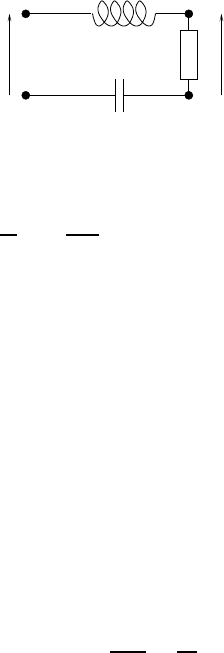
For deﬁniteness, let us look at the very pedestrian example of an electrical

circuit of RLC type (Resistors, Inductors, Capacitors). Assume that the input

signal is the circuit voltage t 7→ u(t), and the output signal is the resistor

voltage t 7→ v(t) (i.e., up to the factor R, the intensity of current in the

circuit).

For instance, a mechanical system with springs and masses, or an elec tric circuit built out

of linear components such as resistors, capacitors or inductors, or in the study o f the free

electromagnetic ﬁeld, ruled by the Maxwell equations.

356 Physical applications of the Fourier transform

u(t) v(t)

Writ ing down the differential equation linking u and v, we obtain the

identity (valid in the sense of distributions):

u =



′

H + δ



∗v = D ∗ v,

which may b e inverted (using the whole apparatus of Fourier analysis!) to

yield an equation of the type

v(t) = T (t) ∗u(t),

where T is th e impulse response of the system, that is, T = D

∗−1

Let us restrict our attention to the case where the input signal is sinusoidal,

with pulsation ω (or frequency ν related to ω by ω = 2πν). The output signal

is assumed to be sinusoidal, with same pulsation ω. The equations are much

simpliﬁed because, formally, we have

“d/dt = iω”

(a differential operator is replaced by a simple algebraic operation). Deﬁne the

transfer function Z(ω) as the ratio between the output signal v(t) = v

iωt

and the input signal u(t) = u

iωt

Z(ω) =

v(t)

u(t)

When the input signal is a superposition of sinusoidal s ignals (which is, gen-

erally speaking, always the case), the linearity of the system may be used to

ﬁnd th e output signal: it sufﬁces to multiply each sinusoidal component of the

input signal by the value of the transfer function for the given pulsation and

to sum (or integrate) over the whole set of frequencies:

if u(t) =

iω

, then v(t) =

Z(ω

) e

iω

and if u(t) =

a(ω) e

iωt

dω, then v(t) =

a(ω) Z(ω) e

iωt

dω.

The only subtle point in this argument is to justify tha t the output signal

is monochromatic if the input signal is. T his step is provided by the following

theorem:

THEOREM 13.1 Any exponential signal (either real t 7→ e

−p t

or c omplex t 7→

2πiνt

) is an eigenfunction of a convolution operator.

Appel W. Mathematics for Physics and Physicists

Подождите немного. Документ загружается.