Alfred DeMaris - Regression with Social Data, Modeling Continuous and Limited Response Variables

Подождите немного. Документ загружается.

variables. The logistic population-growth model, the exponential model with addi-

tive errors, and model D are all essentially nonlinear models. Estimating these mod-

els requires the use of nonlinear least squares, which also depends on the assumption

that model errors are independent and normal, with zero mean and constant variance

(Fox, 1997; Greene, 2003; Neter et al., 1985) This technique is discussed in the ﬁnal

section of this chapter.

COMMON NONLINEAR FUNCTIONS OF X

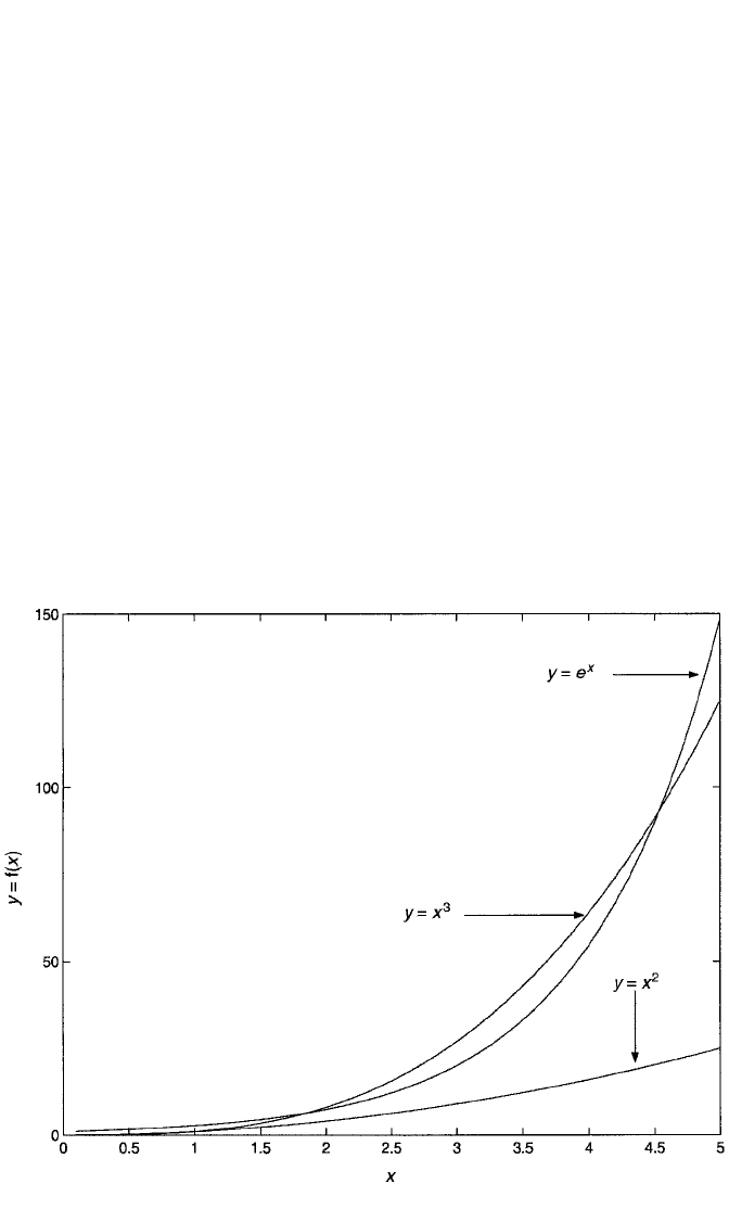
Figures 5.1 to 5.4 present several functions of X that are useful in modeling a non-

linear relationship with Y. These are all curves with one “bend” for X in the range

[0,), and represent the most frequently encountered patterns of nonlinearity. I iden-

tify the curves by linking them to the shapes of the corresponding segments of a cir-

cle that has been quartered. Figure 5.5 illustrates this idea. That is, if we divide a

circle in half by running a line through its middle from left to right, and then divide

it in quarters by running a line through its middle from top to bottom, the circle is

separated into four segments. Segment I is the upper right-hand quarter of the circle,

segment II is the lower right-hand quarter, segment III is the lower left-hand quarter,

COMMON NONLINEAR FUNCTIONS OF X 165

Figure 5.1 Nonlinear relationships exempliﬁed by the functions y  x

, y  x

, and y  e

c05.qxd 8/27/2004 2:52 PM Page 165

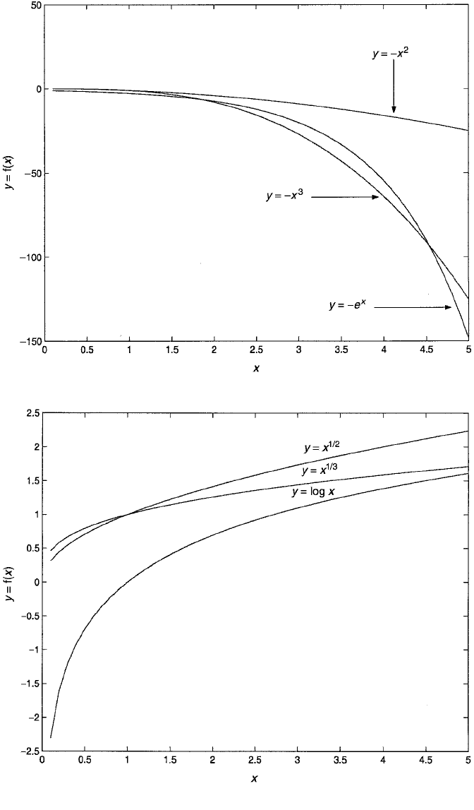
Figure 5.2 Nonlinear relationships exempliﬁed by the functions y x

, y x

, and y e

Figure 5.3 Nonlinear relationships exempliﬁed by the functions y  x

1/2

, y  x

1/3

, and y  log x.

c05.qxd 8/27/2004 2:52 PM Page 166

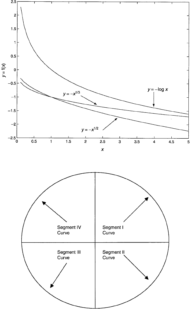
Figure 5.4 Nonlinear relationships exempliﬁed by the functions y x

1/2

, y x

1/3

, and y log x.

Figure 5.5 Segment I, II, III, and IV curves.

c05.qxd 8/27/2004 2:52 PM Page 167

and segment IV is the upper left-hand quarter. The curves in Figures 5.1 to 5.4

resemble these circle segments.

Figure 5.1 presents three functions of X representing segment II curves. These are

all curves with positive slopes, or ﬁrst derivatives, that become more positive with

increasing X. The curve with the most rapidly increasing slope is y  e

, whose

derivative is e

. A slightly less dramatic increase in slope is seen in the curve y  x

Its derivative is 3x

. Finally, a curve with a relatively gentle increase in slope with

increasing X is y  x

, whose derivative is 2x. Figure 5.2 shows some segment I

curves. These can be obtained by simply “reﬂecting,” or changing the sign of, the

functions in the second segment. Notice that all of these curves have negative slopes

that become more negative with increasing X. Figure 5.3 illustrates three segment IV

curves. All of these have the characteristic of having positive slopes that become less

positive with increasing X. This is also easily seen by examining the slopes them-

selves. The most dramatic change, at least in the range of X shown here (.1 to 5) is

exhibited by y  log x. Its slope is 1/x, which ranges from 1/.1  10 to 1/5  .2 in the

ﬁgure. The curve represented by y  x

1/3

appears to “ﬂatten out” most quickly. Its

derivative is 1/3x

2/3

. Its slope ranges from 1.55 when X is .1 to .11 when X is 5. The

curve y  x

1/2

shows a similar pattern but with a more gentle reduction of the slope

with increasing X. Finally, Figure 5.4 presents segment III curves. These curves all

have negative slopes that become less negative with increasing X. Once again, they

can be produced by reﬂecting the three segment IV curves.

Quadratic Functions of X

Although Figures 5.1 to 5.4 present a variety of functions of X that can be used to ﬁt

curvilinear relationships with Y, an especially useful function is the quadratic func-

tion, y  x

. Actually, the correct functional form of a quadratic model for Y is

Y  β

 β

X  β

 ε. (5.1)

This model includes the linear component of X, β

X, along with the curvilinear

component, β

. As Aiken and West (1991) explain, models with higher-order

functions of X should always contain all lower-order components of the higher-

order terms. As these components are often highly correlated with the higher-order

terms, omitting them introduces a type of bias into the equation. That is, the regres-

sion of Y on X

alone might produce a signiﬁcant coeﬃcient for X

due to the cor-

relation between X and X

along with a signiﬁcant eﬀect of X. In this case, the

supposed quadratic eﬀect would be “driven” by a signiﬁcant linear trend that is cor-

related with X

. A true test of whether there is a curvilinear component to the X–Y

relationship is achieved only when we control for X simultaneously. In Aiken and

West’s words: “. . . higher order terms actually represent the eﬀects they are intended

to represent if and only if all lower order terms are partialled from them...”(1991,

p. 110; emphasis in original).

For equation (5.1), d(Y)/dx  β

 2β

X. In this expression, β

encapsulates the

linear component of the curve while β

captures the departure from linearity. In fact,

168 MODELING NONLINEARITY

c05.qxd 8/27/2004 2:52 PM Page 168

if β

 0, there is no departure from linearity, and we are left, once again, with a lin-

ear relationship between Y and X. The signs of β

and β

typically reveal the nature

of the curvilinear relationship between Y and X. For example, let’s assume that X is

always 0. If the X–Y relationship is characterized by the shape of a segment II

curve, both β

and β

should be positive. This indicates that the slope starts out pos-

itive (when X  0) and becomes increasingly positive with increasing X. A segment

I curve would be indicated by both β

and β

being negative. That is, the slope starts

out negative and becomes increasingly so with increase in X. For a segment IV

curve, we would expect β

to be positive and β

to be negative. That is, the slope is

initially positive but becomes less so as X increases. Hence the 2β

X component

of the slope adds an increasingly negative number to β

to bring the overall size of

the slope down ever further with increasing X. Finally, the segment III curve would

be indicated by the opposite pattern: β

should be negative and β

should be posi-

tive. The slope starts out negative, but we add an increasingly positive number

(2β

X) to β

, which has the eﬀect of making the slope less and less negative with

increasing X.

Figures 5.1 to 5.4 do not represent the only possible curvilinear patterns that the

X–Y relationship might exhibit. In particular, they represent relationships between

Y and X that are monotonic in nature. That is, Y is always either increasing (in

segments II and IV) or decreasing (in segments I and III) with X in each case.

Fitting a model that is linear in X in these situations does not lead one too far astray,

since each of these curves could be—at least roughly—approximated by a straight

line. The correlation between Y and X in all cases should be signiﬁcantly nonzero.

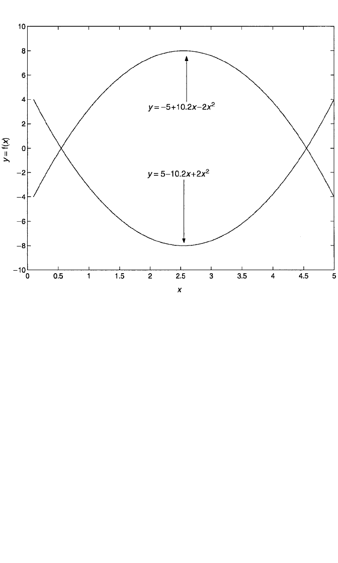
Not so with the curves in Figure 5.6. These are U-shaped (bottom curve) and

inverted U-shaped (top curve) curvilinear relationships that are not monotonic. In

each case, Y is increasing with X over part of X’s range, and decreasing with X over

the rest of X’s range. Fitting a model that is linear in X in these cases is likely to be

very misleading, producing a correlation close to zero. However, a quadratic model

nicely captures this type of curve. As shown in the ﬁgure, each curve was, in fact

generated by a quadratic model. The U-shaped curve has a negative β

and a positive

, while the inverted U-shaped curve shows the opposite pattern. The only way the

analyst can tell whether the data evince the pattern in Figure 5.6, as opposed to

the patterns in Figures 5.3 and 5.4 (segment IV and III curves), is either to graph the

ﬁtted values from the model against X or to plug some sample values of X into the

expression β

 2β

A quadratic model is just a special case of a polynomial model in X. The Jth-order

polynomial model in X is

E(Y )  β

 β

X  β

 β

β

A Jth-order polynomial will ﬁt any curve with J  1 bends. As we have seen, the sec-

ond-order polynomial, the quadratic equation, will ﬁt any curve with one bend. For

a curve with two bends, we could try the third-order polynomial, or cubic equation:

E(Y )  β

 β

X  β

 β

. (5.2)

COMMON NONLINEAR FUNCTIONS OF X 169

c05.qxd 8/27/2004 2:52 PM Page 169

Polynomials higher than second order are rarely used, however. Adding increasingly

higher powers of X tends to produce severe collinearity problems, making estimation

quite unreliable (more about multicollinearity in Chapter 6). Moreover, higher-order

models become increasingly cumbersome to interpret. For example, for equation

(5.2), d(Y )/dx  β

 2β

X  3β

. This suggests that the slope of the X–Y rela-

tionship is itself a quadratic function of X. Not only is this somewhat diﬃcult to

grasp, but it is hard to imagine many theories precise enough to allow the forecast-

ing of such a trend in advance. Most of the time, the quadratic function of X will be

suﬃcient to capture the types of nonlinear relationships found in the social sciences.

(An exception is discussed below, however.)

Applications of the Quadratic Model

To illustrate the ﬁtting and interpretation of models that are nonlinear in X, I consider

the quadratic model in some detail. The GSS98 dataset contains information about

a respondent’s sexual frequency in the last year (coded 0  “not at all” to 6  “more

than 3 times a week”), his or her age (in years), and his or her health (coded 1  “poor”

to 4  “excellent”). [Note that although age is approximately continuous, sexual

170 MODELING NONLINEARITY

Figure 5.6 U-shaped and inverted U-shaped functions of the form y  a  bx  cx

c05.qxd 8/27/2004 2:52 PM Page 170

frequency and health are not. Nevertheless, they will be treated as such, since Bentler

and Chou (1988) suggest that as long as a quantitative variable has at least four cate-

gories, it is safe in analyses to treat it as continuous.] In earlier work with a diﬀerent

sample (DeMaris, 2002b) I have found that there is a nonlinear relationship between

age and sexual frequency which can be captured by a quadratic model. Intuitively, one

would expect that sexual activity would decline with advancing age but that this

decline would not be linear. Age should have a relatively modest negative impact on

sexual activity until after age 50 or so, at which time a decline in testosterone levels,

particularly in men, should accelerate the decline in sexual activity with advancing age.

That is, I expect the relationship between age and sexual frequency to exhibit a seg-

ment I curvilinear pattern such as those in Figure 5.2.

One means of examining relationships for nonlinearity is via the scatterplot. (In

a multivariate context, one might prefer to examine partial plots, in which other vari-

ables have been controlled.) Let’s begin by examining a scatterplot of sexual fre-

quency with respondent’s age, which is depicted in Figure 5.7. A problem that arises,

particularly with discrete response variables having relatively few categories, is that

the scatterplot is not very informative. As is evident, it is diﬃcult to discern any pat-

tern in the relationship between the two variables. An alternative strategy is to parti-

tion a continuous X into intervals and then to plot the mean of Y for cases in each

interval against the interval number. In the current case, I partitioned age according

to deciles of its distribution, with each decile containing approximately 10% of the

2320 respondents. Within each decile, I computed the mean of respondents’ sexual

COMMON NONLINEAR FUNCTIONS OF X 171

Figure 5.7 Scatterplot of frequency of having sex with respondent age for 2320 respondents in the

1998 GSS.

c05.qxd 8/27/2004 2:53 PM Page 171

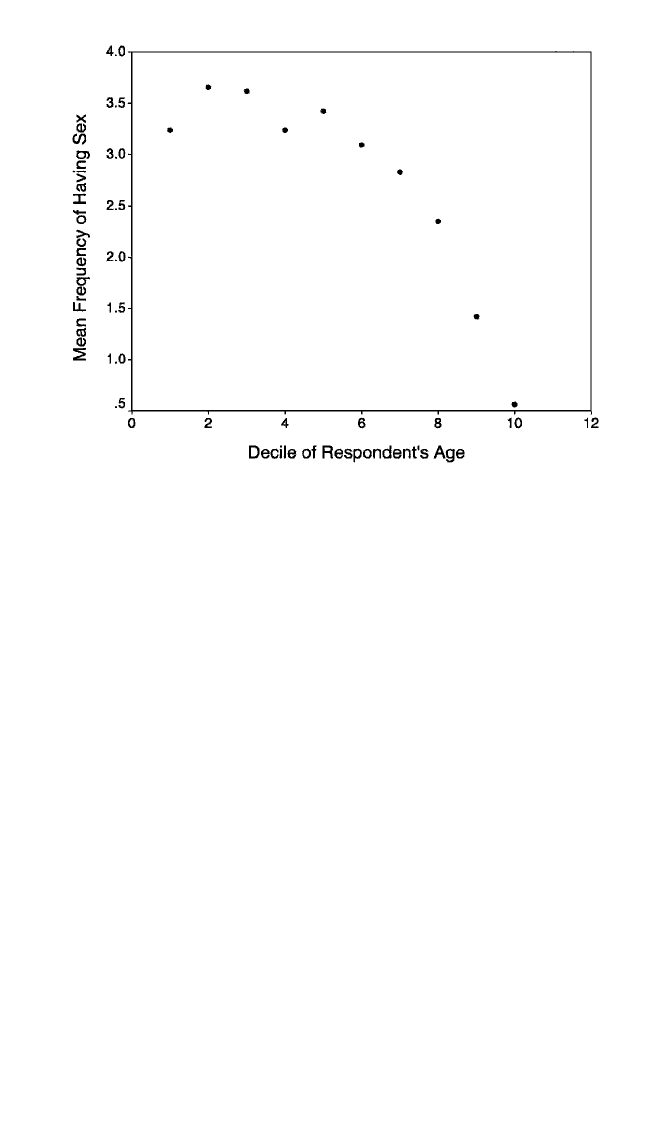
frequencies. A plot of mean sexual frequency with decile of respondent’s age is

shown in Figure 5.8. As expected, the plot resembles the types of curves found in

Figure 5.2: There is a nonlinear decline in mean sexual frequency with advancing

age, with the decline getting ever steeper as age increases. The decline is particularly

swift after the sixth decile, which represents ages 42–47. The curvilinear pattern also

poses some irregularities compared to the curves in Figure 5.2. For one thing, there

appears to actually be an increase in sexual frequency with age at the lowest ages,

followed by a decrease from the third decile (ages 30–34) on. However, this pattern

is easily handled with a quadratic model. Additionally, the fourth decile (ages 34–38)

appears to represent a departure from the general trend of increase followed by

accelerating decline. Whether this is worth taking into account in the model depends

on whether there is strong enough theoretical underpinning to support it. In the cur-

rent case, I treat it as a sample anomaly and assume that a quadratic function is most

appropriate.

Testing Departures from Linearity

As a ﬁrst step in modeling sexual frequency as a function of age, I employ a model

that will ﬁt any pattern in the relationship between these two variables. I refer to it

as the unconstrained model, since it does not constrain mean sexual frequency to fol-

low any particular pattern with respect to age. The variable age decile, representing

deciles of respondent age, is coded 1 for the ﬁrst decile to 10 for the tenth decile. If

we dummy up this variable, omitting the ﬁrst decile (i.e., the youngest age group,

172 MODELING NONLINEARITY

Figure 5.8 Scatterplot of mean frequency of having sex with decile of respondent’s age.

c05.qxd 8/27/2004 2:53 PM Page 172

aged 18–25), the unconstrained model simply regresses sexual frequency on the nine

resulting dummies. The model is

E(Y)  δ

 δ



...

 δ

, (5.3)

where D

, D

, ..., D

denote the nine dummies that represent the second through

the tenth deciles of age. The results are shown as model 1 in Table 5.1. The pattern

of the dummy coeﬃcients conﬁrms the trend shown in Figure 5.7. There is an initial

increase in sexual frequency from the ﬁrst to the second age decile, since those in

the second decile have mean sexual frequency that is .416 higher than those in the

ﬁrst decile. After this, there is a steady decline in sexual frequency, which becomes

more and more pronounced at later ages. Again it is clear that the fourth decile is not

quite in sync with this general trend.

At any rate, is the departure from linearity in the age–sexual frequency relationship,

as revealed in model 1, signiﬁcant? That is, might a linear model nevertheless ﬁt the

trend in the data adequately? We can test this with the test for linearity, a nested F test

based on comparison of model 1 with a model utilizing a linear eﬀect for age decile.

This test takes advantage of the fact that a linear version of model (5.3) of the form

E(Y)  α  β age decile (5.4)

is nested inside model (5.3). Why? Recall from the deﬁnition of nesting in Chapter 3

that model (5.4) is nested inside model (5.3) if its parameters can be generated by

COMMON NONLINEAR FUNCTIONS OF X 173

Table 5.1 Dummy Variable, Linear, and Quadratic Models for the Regression

of Frequency of Sex on Age for 2320 Respondents in the 1998 GSS

Regressor Model 1 Model 2 Model 3

Intercept 3.238*** 2.808*** 3.335***

Age decile .277*** .260***

(Age decile)

.065***

Second age decile .416**

Third age decile .378*

Fourth age decile .002

Fifth age decile .182

Sixth age decile .148

Seventh age decile .413**

Eighth age decile .888***

Ninth age decile 1.817***

Tenth age decile 2.676***

RSS 2002.350 1448.369 1954.210

MSE 2.988 3.216 2.999

.225 .163 .220

Note: Age decile is centered, and the quadratic term for age is based on its centered version.

*p  .05. ** p  .01. *** p  .001.

c05.qxd 8/27/2004 2:53 PM Page 173

174 MODELING NONLINEARITY

placing constraints on the parameters in model (5.3). In fact, model (5.4) is produced

from model (5.3) by placing the following constraints on the deltas in model (5.3):

 α  β; δ

 ( j  1)β for j  2, ...,10. To see that this works, let’s take a couple

of examples. The intercept, δ

, in model (5.3) is the mean sexual frequency for those

in the ﬁrst age decile. According to model (5.4), that mean is E(Y )  α  β(1) 

α  β. The parameter δ

in model (5.3) is the diﬀerence in mean sexual frequency

between those in the eighth age decile and those in the ﬁrst. According to model (5.4),

that diﬀerence is α  β(8)  [α  β(1)]  α  8β  α  β  7β, or ( j  1)β for

j  8. The linear model in equation (5.4) is much more parsimonious than equation

(5.3) since it uses only two parameters instead of 10 to model the data. The diﬀerence

in the model degrees of freedom for these two models is, therefore, 8. The results of

estimating equation (5.4) are shown as model 2 in Table 5.1. The test statistic for

whether the linear model is adequate is

(8,2310)

23.175,

which is quite signiﬁcant ( p  .00001). Apparently, a linear model is not adequate to

ﬁt the data here.

Next, I try the quadratic model:

E(Y )  α  β age decile  γ (age decile)

. (5.5)

We can test whether the pattern of nonlinearity in the data is adequately captured by

the quadratic model with a nested test for model (5.5) versus model (5.3), since model

(5.5) is also nested inside model (5.3). The constraints placed on model (5.3) to pro-

duce the model in (5.5) are δ

 α  β  γ; δ

 ( j  1)β  ( j

 1)γ for j  2, ...

,10. Again a couple of examples reveal why this works. The mean sexual frequency

for those in the ﬁrst decile, according to equation (5.3), is δ

. According to equation

(5.5), it is α  β(1)  γ (1

)  α  β  γ; and δ

in model (5.3) is the diﬀerence in

mean sexual frequency between the ﬁfth and ﬁrst deciles. According to model (5.5),

that diﬀerence is α β(5) γ(5

)  (α  β  γ)  4β  24γ, or ( j  1)β  ( j

 1)γ,

where j  5. As the quadratic model replaces the 10 parameters in equation (5.3) with

only three parameters, the diﬀerence in model degrees of freedom between these two

models is 7. The test statistic for adequacy of the quadratic model is

(7,2310)

2.302.

This is just signiﬁcant at p  .03, which suggests that the quadratic model is not quite

adequate to capture all of the nonlinearity in the age–sexual frequency relationship.

However, in terms of discriminatory power, the quadratic model is a substantial

improvement over the linear model (the change in R

is .057) and only slightly less

eﬃcacious than the unconstrained model (the change in R

is .0054). Adding perhaps

a cubic term might produce a nonsigniﬁcant nested F test, but I do not believe the

(2002.350  1954.210)/7



2.988

(2002.350  1448.369)/8



2.988

c05.qxd 8/27/2004 2:53 PM Page 174