Zelditch M.L. (и др.) Geometric Morphometrics for Biologists: a primer

Подождите немного. Документ загружается.

chap-11 4/6/2004 17: 27 page 278

278 GEOMETRIC MORPHOMETRICS FOR BIOLOGISTS

(A)

(B)

(C)

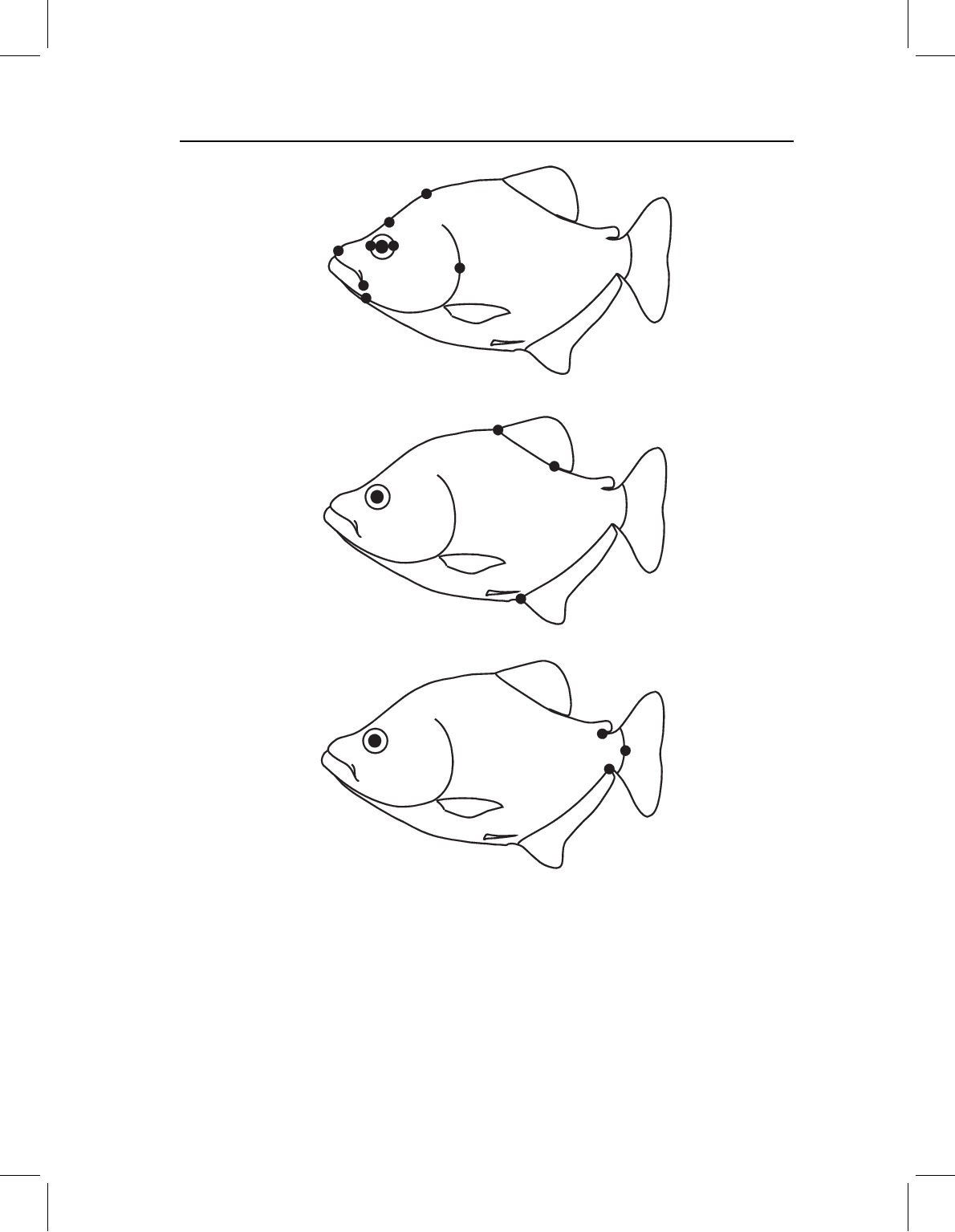
Figure 11.11 Landmarks subdivided into three blocks: (A) cranial; (B) midbody median fins;

We thus separate the landmarks into three blocks: (1) cranial, comprising landmarks

1, 2, 3, 12, 13, 14, 15, 16; (2) midbody median fins, comprising landmarks 4, 5, 9; and

(3) caudal, comprising landmarks 6, 7, 8 (Figure 11.11). Landmark 8 is the posterior

base of the anal fin, so it might seem appropriate to include it in the median fin block;

however, this landmark does not provide any information about body depth, distinguishing

it from the landmarks included in that block. Landmarks 10 and 11 are on the paired fins;

because they do not belong to any of the blocks singled out by this hypothesis, they are

chap-11 4/6/2004 17: 27 page 279

PARTIAL LEAST SQUARES ANALYSIS 279

excluded from the analysis. We will examine the integration between the cranial landmarks

and each of the other two blocks, producing two pairs of blocks with the cranial landmarks

being included in both pairs.

The correlation between cranial and tail landmarks is very high in S. gouldingi

(R =0.888), as is the correlation between cranial and fin landmarks (R =0.751). To deter-

mine if one correlation is higher, we need to determine whether the difference between the

two correlations is larger than we would expect by chance. There are two ways to test this

hypothesis: one is to compare the difference between the correlations to the standard error

of the difference; the other is to bootstrap the difference between correlations and ask if the

95% range of the difference includes zero. Based on the first (analytic) approach we would

reject the null hypothesis that the correlations are equal (p =0.011), but, because the test

presumes normality, we ought to check the result using a resampling-based method. The

95% range for the difference between correlations is −0.262 to −0.0342, which excludes

zero and also leads us to reject the null hypothesis of equal correlations. Thus we conclude

that cranial and tail landmarks are more highly integrated with each other than are cranial

and median fin landmarks.

The analysis of S. manueli reveals a different pattern. In this species, both correlations

are weak: that between cranial and tail landmarks is R =0.443, and that between cranial

and median fin landmarks is R =0.599. The analytic test of the difference between cor-

relations indicates that the two correlations differ by no more than expected by chance

(p =0.251), as does the resampling-based test (the 95% interval of R is −0.366 to +0.134,

which includes zero). This contrast between integration patterns of S. manueli and S.

gouldingi is expected in light of their different ontogenetic allometries; we would need to

devise a timing hypothesis for S. manueli that does not follow the expected spatiotemporal

pattern. An interesting subject to pursue further is whether we can use studies of allom-

etry to infer patterns of timing that accurately predict developmental correlations among

blocks.

Using PLS to relate shape to ecological factors

We now use PLS to examine the relationship between shape and a block of non-shape

variables, specifically latitude and longitude. We will examine geographic variation in

adult body shape in a widely distributed piranha species, Pygocentrus nattereri. Geo-

graphic variation is often analyzed using conventional ordination methods like PCA, so

we will analyze the same data using both PCA and PLS. To simplify the analysis we

restrict the sample to the northern populations, because the southernmost ones might

belong to a different species (an inference difficult to make from morphology without a

detailed analysis of geographic variation). Also, we exclude the smallest specimens to avoid

confounding geography with ontogeny. We could conceivably include all the specimens,

standardizing shape statistically (using the regression equation for shape on size), but that

procedure assumes that deviations from the regression are equal across the entire size

range. Violating that assumption could distort the covariance structure of shape, which

could complicate the analysis of geographic variation. Therefore we limit this analysis

to the 48 largest specimens of P. nattereri, which still includes considerable variation in

size: individuals range from 102 mm to 225 mm standard length. Before we can interpret

chap-11 4/6/2004 17: 27 page 280

280 GEOMETRIC MORPHOMETRICS FOR BIOLOGISTS

⫺0.03

⫺0.02

⫺0.01

0.01

0.02

0.03

⫺0.04 ⫺0.03 ⫺0.02 ⫺0.01 0 0.01 0.02 0.03 0.04 0.05

PC1

PC2

18–19

3–5

Degrees south

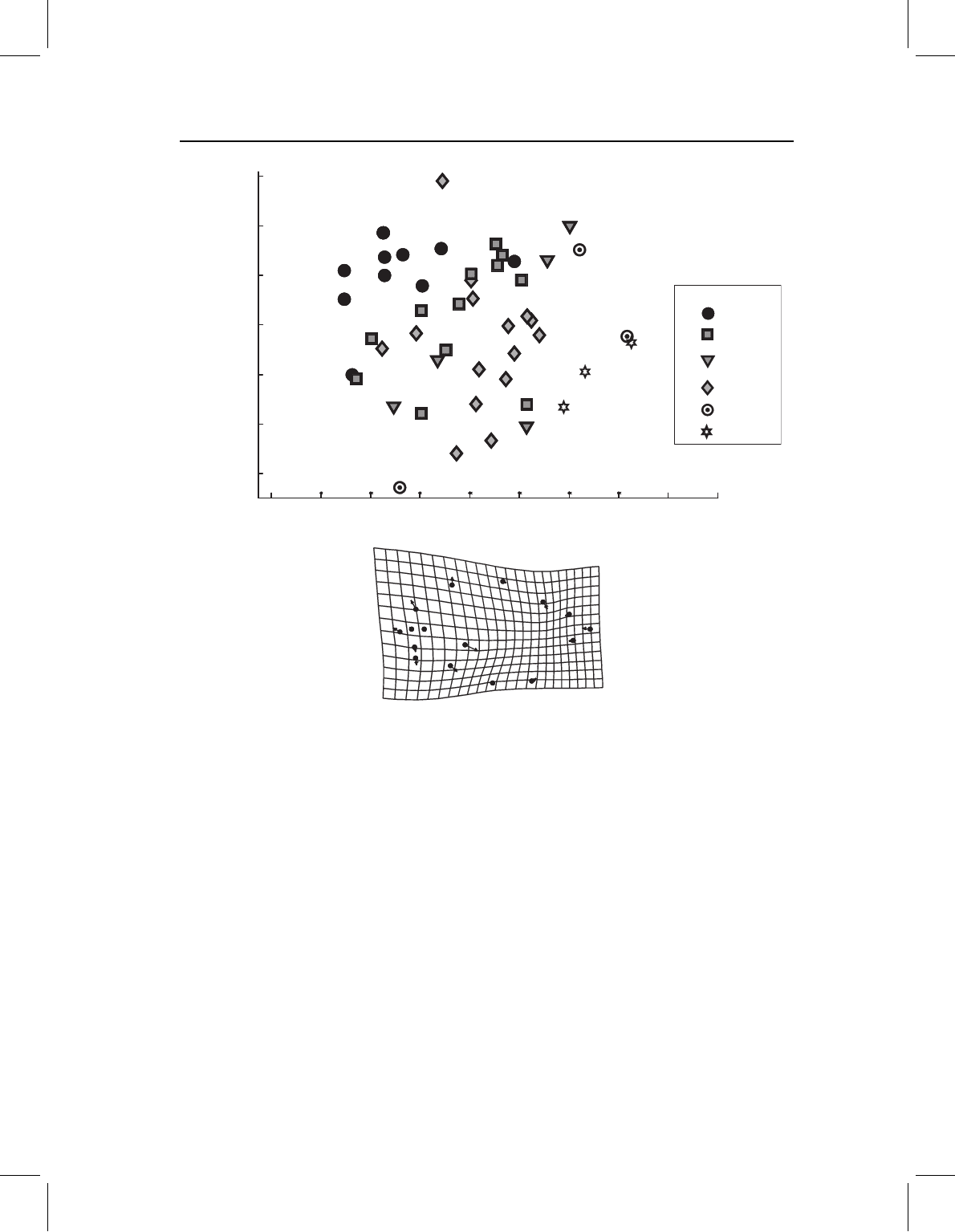
Figure 11.12 Principal components of shape variation of P. nattereri, specimens coded to indicate

latitude where collected. The deformation grid depicts the shape transformation in the direction of

higher scores on PC1, which is towards the more southerly localities.

the covariance between shape and geography, we will have to determine whether that

covariance could instead be due to a covariance between size, shape and geography.

PCA of P. nattereri shape

The analysis of whole body shape by PCA yields no distinct eigenvalues: PC1 accounts

for just 18.1% of the variance, PC2 accounts for 15.1%. Although the variation has no

dominant direction, there is a slight hint of a geographic pattern in the scores on PC1

(Figure 11.12). Although the evidence is hardly compelling, the specimens collected in the

northern localities are generally towards the left of the plot, whereas those collected in

the most southern localities are generally towards the right. We thus tentatively explain

PC1 as a latitudinal gradient in shape: southern P. nattereri tend to have larger heads

for their bodies (especially relative to the most posterior body). However, the evidence

is not compelling. The analysis of the cranial landmarks provides even less evidence for

chap-11 4/6/2004 17: 27 page 281

PARTIAL LEAST SQUARES ANALYSIS 281

⫺0.06

⫺0.04

⫺0.02

0.02

0.04

⫺0.08 ⫺0.06 ⫺0.04 ⫺0.02 0 0.02 0.04 0.06 0.08

PC2

PC1

18–19

3–5

Degrees south

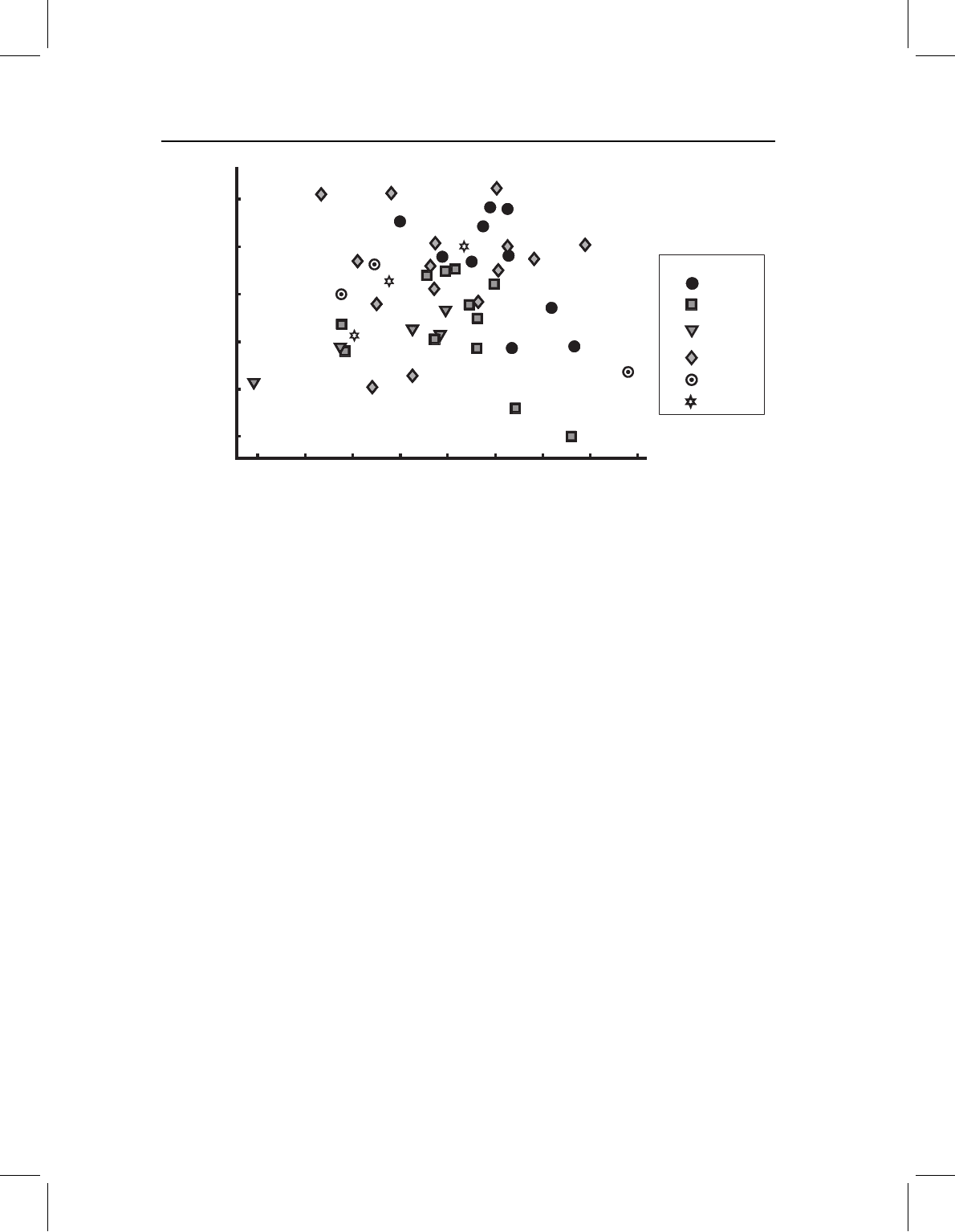
Figure 11.13 Principal components of cranial shape variation of P. nattereri, specimens coded to

indicate latitude of the locality where the individual was collected.

any geographic trends (Figure 11.13). Again there are no statistically distinct eigenvalues,

although PC1 accounts for 31% of the variance and PC2 for only 18.4%. Individuals from

the northernmost locality appear to be scattered fairly evenly over the entire plane. Four

individuals from the southernmost localities are concentrated to the left, but two other

specimens from southern localities are towards the right. The variation in postcranial

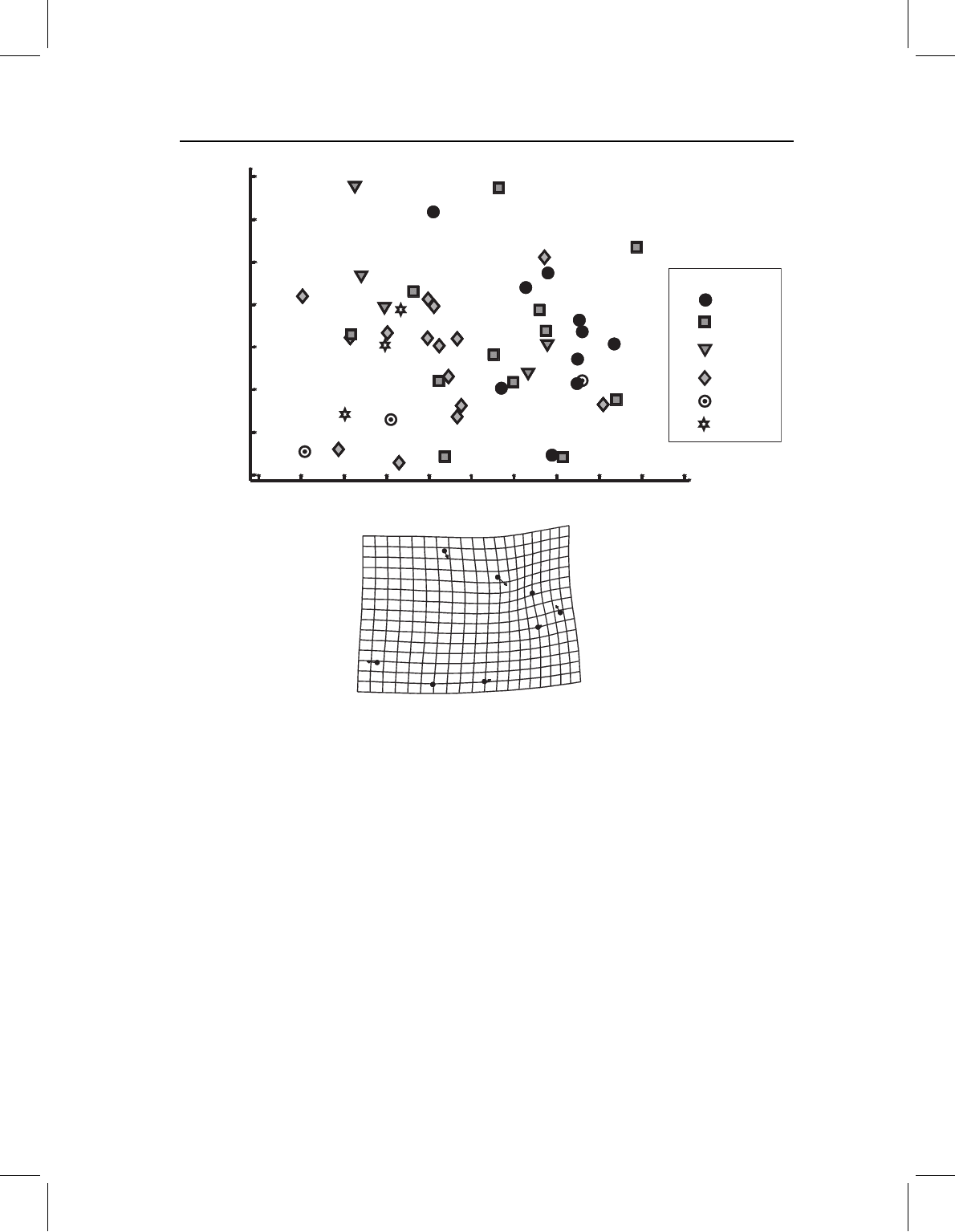
shape also lacks a dominant direction, although PC1 explains 28.9% of the variance and

PC2 explains 16.2% of the variance (Figure 11.14).

Compared to cranial shape, postcranial shape offers a stronger hint of a geographic

pattern because individuals from the northernmost localities are generally concentrated to

the right of the plot of PC2 on PC1 whereas those from the southernmost localities are

generally to the left. Based on Figure 11.13, we might thus interpret PC1 tentatively as

indicating a latitudinal gradient in postcranial shape; more southern P. nattereri tend to

have a longer dorsal fin base relative to the length of the posterior body.

PLS: the covariance between P. nattereri shape and geography

When we explicitly examine the covariation between shape and geography for whole body

shape, PLS extracts one dimension of covariance (with a singular value of 0.0493) explain-

ing 46.6% of the covariance between the two blocks. Interestingly, the one statistically

significant singular value is the second; the first, with a value of 0.0564, does not explain

more covariance than expected by chance. The loadings of the two geometric variables

suggests that this is a longitudinal factor, and the reason why this may not be signifi-

cant is that there is a small number of eastern Brazilian specimens that might differ from

the more easterly populations (for reasons unrelated to a longitudinal trend). SA2 does

account for significantly more covariance than expected by chance (p < 0.01), and the

chap-11 4/6/2004 17: 27 page 282

282 GEOMETRIC MORPHOMETRICS FOR BIOLOGISTS

PC1

PC2

⫺0.03

⫺0.02

⫺0.01

0.01

0.02

0.03

0.04

⫺0.05 ⫺0.04 ⫺0.03 ⫺0.02 ⫺0.01 0 0.01 0.02 0.03 0.04

0.05

18–19

3–5

Degrees south

Figure 11.14 Principal components of postcranial shape variation of P. nattereri, specimens coded

to indicate latitude where collected. The deformation grid depicts the shape transformation in the

direction of lower scores on PC1, which is towards the more southerly localities.

correlation between the blocks (of 0.77) is also statistically significant. Before going any

further, we need to check whether this correlation between geography and shape might be

confounded by a correlation between shape and size. The evidence against this hypothesis

is in the weak (non-significant) correlation between scores on SA2 and size (R =−0.093).

Thus we can proceed to interpret SA2 as a possible geographic factor, bearing in mind that

SA2 is defined to be independent of SA1, and SA1 is not significant (and may be heavily

influenced by the easternmost specimens).

Only latitude makes a large contribution to SA2; its loading is 0.993 whereas that of

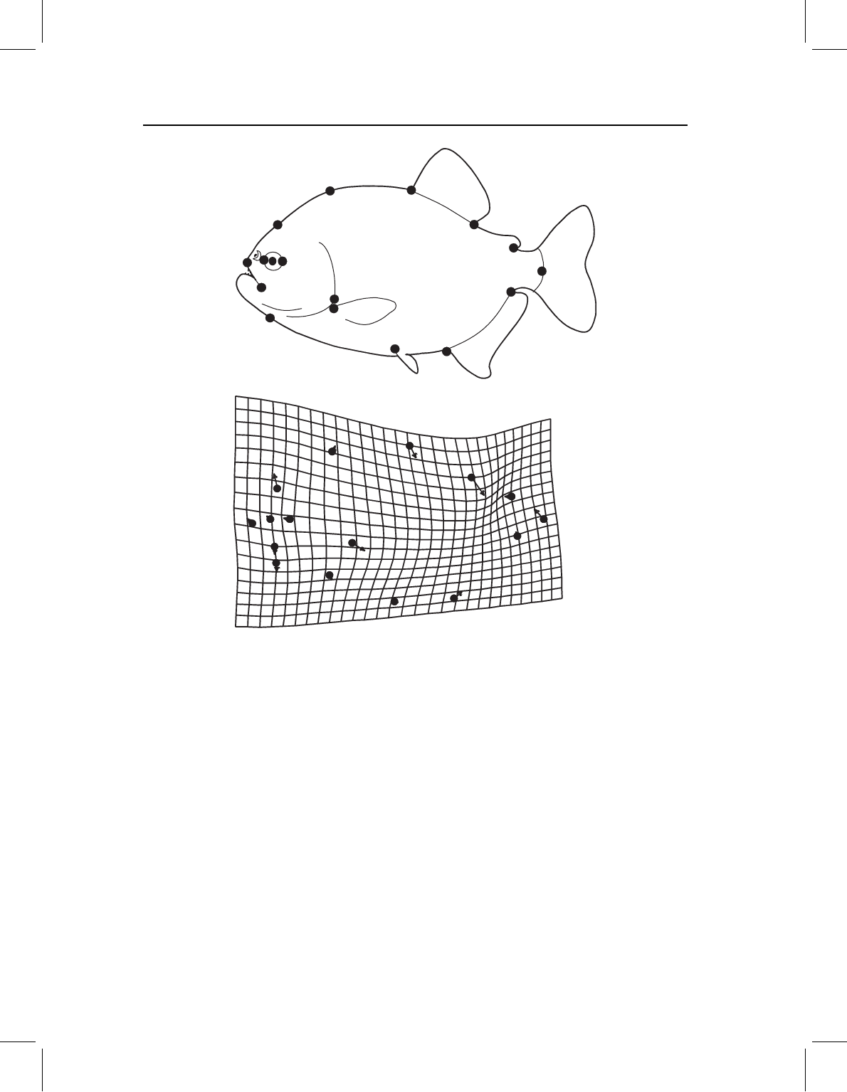
longitude is only 0.117. Figure 11.15 shows the shape covariate of latitude (depicting

the transformation in the whole shape moving southerly): a marked increase in head size

relative to that of mid- and posterior body (especially relative to the region between dor-

sal and adipose fins), with steepening of the anterior head profile and shallowing of the

more posterior head profile (producing a generally blunter head), and an expansion of

the postorbital region.

chap-11 4/6/2004 17: 27 page 283

PARTIAL LEAST SQUARES ANALYSIS 283

Figure 11.15 The covariance between P. nattereri shape and geography, depicted as a transforma-

tion in the southerly direction.

In the analysis restricted to cranial landmarks we again find that the second singular

value, 0.0606, is significant. SA2 explains 31% of the covariance between geography and

shape. The correlation of 0.59 is moderately high and statistically significant (p < 0.01).

SA2 does not appear to be confounding size and geography, because the correlation

between scores on SA2 and size is non-significant (−0.152; p < 0.05). Again the geo-

graphic factor is dominated by latitude: the loading of latitude on SA2 is 0.99, whereas

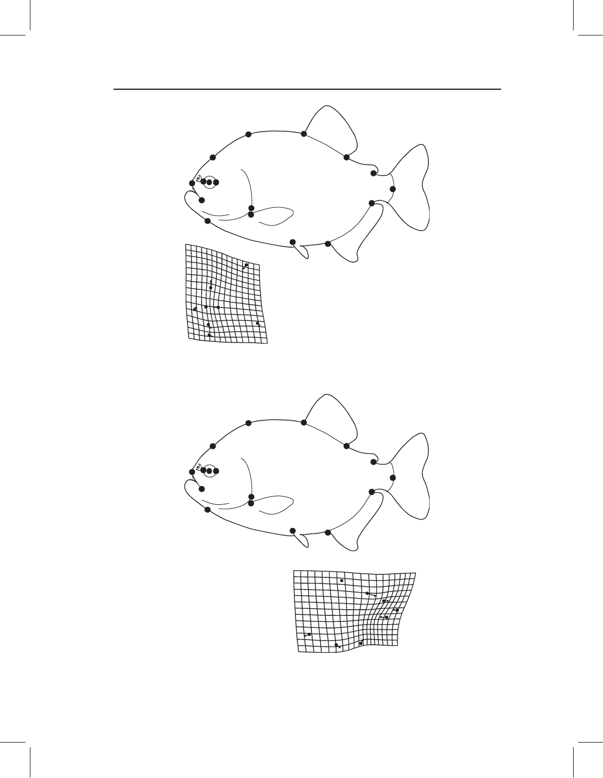
that of longitude is only 0.16. Figure 11.16 shows the shape covariate of latitude (again

depicting the transformation in shape when moving southerly). As in the analysis of whole

body form, there is steepening of the anterior head profile and shallowing of the more

posterior head profile (producing a generally blunter head), and also a slight lengthening

of the postorbital head relative to eye diameter. Because the analysis is restricted to the

cranial landmarks, we cannot see the general increase in head length relative to the mid-

and posterior body.

In the analysis restricted to postcranial landmarks we find a strikingly different pattern,

although the salience of geography for shape is still apparent. As before, there is only one

chap-11 4/6/2004 17: 27 page 284

284 GEOMETRIC MORPHOMETRICS FOR BIOLOGISTS

Figure 11.16 The covariance between P. nattereri cranial shape and geography, depicted as a

transformation in the southerly direction.

Figure 11.17 The covariance between P. nattereri postcranial shape and geography, depicted as a

transformation in the southeasterly direction.

chap-11 4/6/2004 17: 27 page 285

PARTIAL LEAST SQUARES ANALYSIS 285

significant singular value; the second (0.050), which accounts for 46.4% of the covariance

between shape and geography. The correlation between postcranial shape and geography

is relatively low (R =0.40), but it is an interesting composite of latitude and longitude.

The loading for latitude is 0.617 and that of longitude is −0.717, so the two geographic

directions are nearly equal and inversely related. Figure 11.17 shows the transformation

in postcranial shape moving southeasterly: a shortening of the body posterior to the dorsal

fin (especially of the anal fin), which is in contrast to a slight elongation of the region

between pectoral and pelvic fins.

Software

Two programs in the IMP series perform partial least squares analysis. One is designed

to analyze a single population (PLSMaker), as in the analyses of developmental inte-

gration within species and in the analysis of geographic variation of P. nattereri; the

other (PLSAngle) is used for comparative studies, including comparisons between species

and comparisons between correlations of blocks (as in the analysis of correlations

between cranial and tail versus cranial and median fin landmarks in S. gouldingi and

S. manueli).

Both programs take input files of landmark coordinates in standard X1,Y1…CS format.

One block can be non-landmark data, which should be formatted so that all measurements

for each specimen are in the same row and the specimens are in the same order as they

are in the file of landmark data. Both programs perform a GLS superimposition prior

to computing SAs, so the superimposition used to produce the input file of landmark

coordinates does not matter.

Running PLSMaker

To load the first block of data, which must be landmarks, click on the Load Data button.

The second block can comprise any non-landmark data; if that is what you are loading,

click on the radio button in the second block next to Landmark Data (which will turn

off the default). You will notice that there is a third field, to allow for loading a third

block of data; this option is not yet enabled (check for upgrades). When the data are

loaded, they will appear in the visualization window to the left. You can see those plots

again by clicking on the Show Data buttons located within the field for each block below

Load Data.

To perform a two-block PLS, click on the 2Block SVD button below the Load Data

fields. The numerical results will appear in the orange field at the bottom, although only

the results for the first singular value and axis will initially be displayed. To look at those

for the second (and subsequent) axes, move Up or Down the Active SVD Axes. You will

see the singular value (SVD score), the percent covariance explained (SVD percentage),

and the correlation between blocks explained by that axis.

To determine which, if any, of the singular values and correlations are significant,

use the Statistics pull-down menu on the toolbar. At present, there is only one option

(Permutation Test). The default is to do 100 permutations, so if you wish to do more,

type in the number in the box under # of Permutations (located in the purple field of the

chap-11 4/6/2004 17: 27 page 286

286 GEOMETRIC MORPHOMETRICS FOR BIOLOGISTS

display options). The results will appear in the auxiliary window. The first results state

the singular value, and the number of times that a value equal to or higher than this was

obtained in the chosen number of random permutations; the final column is the p-value

for the null hypothesis (that this frequency can be explained by chance). The second set

of results, printed below, gives the correlations between the scores of the first and second

blocks for each singular axis, and the number of times that an equal or higher value was

obtained in the chosen number of random permutations; again, the final column is the

p-value for the null hypothesis (that this frequency can be explained by chance). It is

entirely possible that the singular value is not significant but the correlation is. This occurs

when the axis explains a trivial part of the covariance. The results seen in the auxiliary

window can be copied from the window (by selecting the text and copying it using ˆC)

and pasted into a text file (using ˆV) or appended to a file by clicking on the option

Append Results to File. As usual, you can safely ignore the caution about overwriting

the file.

You can see the relationship between the scores of Block 1 and Block 2 by clicking on

Show Scores just below 2Block SVD (both are below the Load Data fields). If both data

sets are blocks of shape data the plot can be copied to the clipboard, but you will need

to use the auxiliary copy function (because the copy function that preserves the aspect

ratio in plots of the shape transformations interferes with copying the plots of the scores).

Alternatively, you can save the scores to files and use the plotting options in Excel (or

another program) by going to the File menu on the toolbar up top and selecting Save

Scores for Block 1 then Save Scores for Block 2.

To depict the singular axes as shape deformations (for landmark data) or as loadings of

the non-shape variables, click on Plot Axis (located in the field for each block, beneath the

Load Data and Plot Data options). You have the usual options for displaying the shape

transformations; some are in the purple field below the visualization window, the remain-

der are listed in the Image pull-down menu on the toolbar up top. In the purple field you

may select Plot Style, the Superimposition method to use when depicting the deformation

(if you select either Bookstein Coordinates (BC) or Sliding Baseline Registration (SBR),

make sure to type in the endpoints of your baseline in the boxes that are provided on the

right side of the purple field). You can multiply the deformation by a factor by typing

that factor into the Exaggeration box, you can alter the range of the grid (if it is too large

or small for your landmarks) by typing the desired range in the Range box, and you can

also alter the Density of the plot (the number of grid lines in the deformed grid plots).

To alter line weights, symbol sizes (and whether empty or filled) and to remove the axes

from the plot, go to the Image menu on the toolbar. As usual, you can trim the grid if

it extends too far beyond the landmarks by clicking on the Grid Trimming Active radio

button, located on the right, and you can rotate the plots by clicking on the Reference

Rotation Active. Because it may be difficult to see how the specimens are oriented when

looking at an unfamiliar subset of landmarks, you have the option of printing the number

for each landmark on the plot. This should help you determine the angle through which

you will need to rotate the plots.

You can save the scores for each SA for each block, and the singular value decomposition

information (the singular values, S-Value, the percentage of the covariance between blocks

explained, Percentage, and the U and V matrices). The files of scores are ordered so that

SA1 is in the leftmost column, SA2 in the one to the right of it, etc.

chap-11 4/6/2004 17: 27 page 287

PARTIAL LEAST SQUARES ANALYSIS 287

Running PLSAngle

Two sorts of comparisons can be made using PLSAngle. The first is between SAs of the same

blocks of landmarks belonging to different groups (i.e. species). In this kind of analysis,

the hypothesis being tested is that the corresponding SAs are the same between groups

(for example, that the SA1 of the cranial landmarks is the same for two species). The

second kind of comparison is between correlations. It is easiest to follow the logic of the

instructions by thinking of the groups as competing hypotheses of integration; one “group”

is the hypothesis that Block 1 and Block 2A are most highly correlated, the other “group”

is the alternative hypothesis that Block 1 and Block 2B are most highly correlated. As well

as asking if one correlation exceeds the other, we can also ask whether SA1 is the same

when Block1 is constant but Block 2 varies (i.e. whether the dominant axis of covariance

between the cranial and tail landmarks is the same dimension as the dominant axis of

covariance between the cranial and median fin landmarks). Finally, PLSAngle also allows

you to visualize PCs and SAs, so you can see if the dimensions of variance are equivalent

to the dimensions of covariance. You can also visually compare the PCs between the two

groups, as well as look at the PCs for each group separately. PLSAngle also displays the

SAs for each block in each group. The program is still under development, so check for

upgrades that offer statistical tests between PCs and SAs.

Comparing singular axes of homologous blocks between groups

The default is that both blocks are homologous. Load the blocks; the landmarks will

appear in the visualization window as each file is loaded. Clicking on the Do SVD (2Block)

button will calculate the angles between the corresponding SAs of the two groups. The

results will appear in the Auxiliary Results box (another window). You will see a list of

results, beginning with the line “SVD 1 Block 1 =21.525 Block 2 =30.534.” This means

that the angle between the SA1 of Block 1 in the two groups is 21.525

◦

, whereas the angle

between the SA1 of Block 2 in the two groups is 30.534

◦

. The next line reports the angles

between SA2 for each block, the third for SA3, and so forth.

Asking to do an SVD will not provide confidence intervals on the angles; to get those,

you will need to click on Bootstrap SVD Angle. The default is to run 100 bootstraps, and

to test the null hypothesis at an α level of 0.05. If you want to increase the number of

bootstraps or lower the alpha level, type in your preferences before clicking on Bootstrap

SVD Angle (Remember that α cannot be lower than 1/N

bootstraps

, where N

bootstraps

is the

number of bootstraps. For example, if you run 100 bootstraps, the smallest value of α you

can request is 1/100, or 0.01.)

You can save the SAs for Block 1 and Block 2 for each group, along with the reference

forms used to compute the partial warp scores. You can also save PC1 for each of the

blocks of each group. The output files are row vectors, the format required by VecDisplay.

If you want to save the SA scores for each specimen, use PLSMaker.

A long list of options for graphical displays is presented in the Display Item menu in

the purple field below the visualization window (although some of the options are not

available if Block 2 is not homologous):

1. SVD Block1, Group1+2 shows SA1 for Block 1 for both groups simultaneously. The

PCs are displayed by pairs of vectors of relative landmark displacements. The vectors