Zdunkowski W., Bott A. Dynamics of the atmosphere: A course in theoretical meteorology

Подождите немного. Документ загружается.

27.1 Derivation and discussion of the Lorenz equations 671

On replacing T

in this expression by T

and α

by α

we obtain the equation of

state for the speciﬁc volume:

α(T ) = α

(1 + T

)(27.8)

where α

is the mean value of the speciﬁc volume of the entire region of convection

and  = 1/T

is the cubic expansion coefﬁcient of the air.

Next we need a suitable expression for the pressure p(x,z, t), which may be

expressed as the sum of the hydrostatic pressure p

(x,z, t) and the deviation



(x,z, t) from this value. Let p

(z, t) represent the horizontal average of the

hydrostatic pressure at height z and time t and

(z, 0) be the initial value at time

t = t

. Furthermore, we introduce a new pressure variable P according to

P (x,z, t) = [p(x,z,t) −

(z, 0)]α

= [p(x,z, t) − p

, 0)]α

− g(z

− z)

with p(x, z,t) = p

(x,z, t) + p



(x,z, t),

(z, 0) = p

, 0) +

− z)

(27.9)

where z

denotes the top of the convective layer. In reality P has dimensions of

energy per unit mass. Thus we may express the Jacobian J (α, −p)by

J (α, −p) = J



(1 + T

), −

− p

, 0) −

− z)



(27.10a)

Expansion of the Jacobian yields

J (α, −p) = J(T

, −P ) + g

∂T

∂x

≈ g

∂T

∂x

(27.10b)

The ﬁrst term on the right-hand side of this expression is of second order in

comparison with the second term and has, therefore, been neglected. By utilizing

(27.10b) in (27.5) we obtain Saltzman’s approximate form of the vorticity equation:

∂

∂t



∇



+ J



ψ, ∇



= g

∂T

∂x

+ ν ∇



∇



(27.11)

This is an equation in two unknowns involving the stream function ψ and the

temperature deviation T

. Therefore, a second prognostic equation is needed in

order to determine T

. In order to avoid the appearance of new dependent variables

Saltzman chooses the very simpliﬁed form of the heat equation

∂T

∂t

+ v

·∇

= K ∇

(27.12)

672 Predictability

where K is the exchange coefﬁcient for heat. Introducing the stream function ψ

according to (27.4), the heat equation can be written in the concise form

∂T

∂t

+ J (ψ, T

) = K ∇

(27.13)

Thus equations (27.11) and (27.13) describe the model convection in the (x,z)-

plane. It should be realized that, due to the appearance of clouds and phase transi-

tions, the actual convective processes are much more complicated.

The temperature deviation T

may be decomposed and expressed as the sum of

an average value

(z, t) along the x-axis plus the deviation T



(x,z, t):

(x,z, t) = T

(z, t) + T



(x,z, t)(27.14)

Furthermore, T

(z, t) can be decomposed into a part representing a linear variation

between the upper and lower boundary and a departure T



from the linear variation:

(z, t) =



(0,t) − T

(t)



+ T



(z, t)(27.15)

with T

(t) = T

(0,t) − T

,t). Now equation (27.14) can be written in the

following form:

(x,z, t) =



(0,t) − T

(t)



+ ϑ(x,z,t)(27.16)

with ϑ(x,z,t) =



(z, t) + T



(x,z, t). Saltzmann assumes that the temperatures

at the lower and upper model boundaries are kept constant by external heating.

This implies

(0,t) = T

(0), T

,t) = T

) =⇒ T

= T

(0) − T

) = constant

(27.17)

so that

∂T

∂t

∂ϑ

∂t

∂T

∂x

∂ϑ

∂x

∂T

∂z

=−

T

∂ϑ

∂z

, ∇

=∇

(27.18)

follow from (27.16) and (27.17). From (27.11) and (27.13) we ﬁnally ﬁnd a pair of

partial differential equations describing the convection

∂

∂t



∇



+ J



ψ, ∇



= g

∂ϑ

∂x

+ ν ∇

(∇

ψ)

∂ϑ

∂t

+ J (ψ, ϑ) =

T

∂ψ

∂x

+ K ∇

(27.19)

27.1 Derivation and discussion of the Lorenz equations 673

The ﬁrst terms on the right-hand sides of (27.19) represent the driving forces of

the convection while the second terms cause damping due to viscosity and heat

conduction.

We wish to introduce the dimensionless Rayleigh number, which is deﬁned by

Ra =

gz

T

νK

(27.20)

Ra is a measure of convective instability. The numerator of Ra involves the buoy-

ancy force per unit mass gT

while the denominator denotes damping expressed

by the kinematic viscosity ν and the heat-conduction coefﬁcient K.Ifz

and l

stand for the height and the width of the convection rolls, the aspect ratio a = z

deﬁnes the critical Rayleigh number

(1 + a

)

(27.21)

The critical Rayleigh number depends on the geometric parameters of the model.

Whenever the ratio r = Ra/Ra

> 1, convection is expected to occur.

Saltzman (1962) assumes that the stream function and the temperature departure

in equation (27.19) can be expressed as sums of double Fourier components.

Lorenz (1963), motivated by Saltzman’s work, assumed the validity of the simple

trial solutions

ψ =

√

2(1 + a

X(t)sin



πax



sin



πz



ϑ =

T

πr



Y (t)

√

2cos



πax



sin



πz



− Z(t)sin



2πz



(27.23)

containing only three development coefﬁcients X(t),Y(t),Z(t), which are slowly

varying amplitudes in time. According to the trial solution, the X mode represents

the ﬂow pattern, the Y mode the temperature cells, and the Z mode the temperature

stratiﬁcation. When equations (27.23) are substituted into (27.19), ignoring trigono-

metric terms that do not occur in the trial solution, we obtain the famous Lorenz

system consisting of three ordinary differential equations in dimensionless time t

∗

X =−σX + σY = f

(X,Y,Z)

∗

Y = rX − Y − XZ = f

(X,Y,Z)

∗

Z = XY − bZ = f

(X,Y,Z)

with t

∗

+ 1)K

t, σ =

,b=

+ 1

> 0,r=

(27.24)

674 Predictability

The term σ is the Prandtl number. The consequence of the simpliﬁcation is that

the advection term in the ﬁrst equation of (27.19) is suppressed.

The Lorenz system is a three-dimensional autonomous dynamic system, which

may formally be expressed by

X = f(X)withX = (X,Y,Z)(27.25)

If the function f depends not only on the vector X but also explicitly on time t,we

speak of a nonautonomous dynamic system. This type of system is more difﬁcult

to handle.

Owing to the simpliﬁcations introduced by Lorenz, this approach does not re-

alistically model convection rolls. What Lorenz had in mind was to show that the

low-order nonlinear dynamic system (27.24) with only three degrees of freedom

reacts very sensitively to small variations in the initial conditions. This simple fact

has many important consequences for weather prediction.

The discussion of simple properties of the Lorenz system requires that the reader

is somewhat familiar with a few basic concepts of nonlinear dynamics. Some

readers may be quite familiar with this subject; others may wish to consult one of

the many textbooks which are available at all levels of sophistication. For the reader

entirely unfamiliar with the subject, we gave a brief and incomplete introduction

in Chapter M7. There we extract most of the required information from Strogatz’s

excellent book on Nonlinear Dynamics and Chaos (1994). His very informative

book is much more than a ﬁrst introduction. It provides pleasant reading at a level

of mathematical sophistication that does not exceed the usual background of a

senior student in meteorology. The next four sections again follow his book.

Inspection of (27.24) shows that the only nonlinearities are the quadratic terms

XY and XZ. Lorenz found that, over a wide range of parameters, the numerical

solutions oscillate irregularly in time, but they never exactly repeat. This led him to

title his now famous paper “Deterministic Non-Periodic Flow”. Moreover, he found

that the solutions to (27.24) always remain in a bounded region of phase space.

When he plotted the trajectories in three dimensions, there emerged a strange ﬁgure

that resembled a pair of butterﬂy wings. This ﬁgure is now called a strange attractor.

In the following we list important simple properties of the Lorenz equations.

27.1.1 Nonlinearity

The Lorenz system consists of the two nonlinearities XY and XZ.

27.1 Derivation and discussion of the Lorenz equations 675

Fig. 27.1 Contraction in volume of a dissipative system.

27.1.2 Symmetry

On replacing (X,Y) in (27.24) by (−X, −Y ), the equations do not change. Thus,

if [X(t

∗

),Y(t

∗

),Z(t

∗

)] is a solution to (27.24), so is [−X(t

∗

), −Y (t

∗

),Z(t

∗

)].

27.1.3 The Lorenz system is dissipative

In general, a dynamic system is either conservative or dissipative. An important

property of phase space is the preservation of phase volume of conservative or

constant-energy systems. For dissipative systems, the volume in phase space con-

tracts under the ﬂow. In this case the divergence of the phase velocity is negative.

In contrast, if the divergence is zero, the dynamic system is conservative.

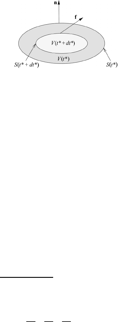
To illuminate the idea, we consider an arbitrary closed surface S(t

∗

)ofthe

volume V (t

∗

) as shown in Figure 27.1. We may think of points on S as initial

conditions for trajectories that evolve during the time interval dt

∗

, thus resulting

in a change in volume. What is the volume at time t

∗

+ dt

∗

? As usual, the vector

n denotes the outward normal on S. We do not have to restrict ourselves to the

Lorenz system, but we consider the arbitrary three-dimensional system

X = f(X).

The scalar product f · n is the outward normal component of the velocity vector

X. During the time interval dt

∗

a patch of surface area dS = n dS sweeps out a

volume element dV = (f · n dt

∗

) dS = V (t

∗

+ dt

∗

) − V (t

∗

). Integrating over all

patches yields

V =

V (t

∗

+ dt

∗

) − V (t

∗

)

∗



f · n dS =



∇·f dV (27.26)

where we have used Gauss’ divergence theorem (M6.31). For the Lorenz system

the divergence ∇·f turns out to be

∇·f =

∂f

∂X

∂f

∂Y

∂f

∂Z

=−(σ + 1 + b) < 0(27.27)

676 Predictability

On substituting this expression into (27.26) we obtain for the change of the

volume with time

V (t

∗

) =−(σ + 1 + b)V (t

∗

)(27.28a)

from which it follows that

V (t

∗

) = V (0) exp[−(σ + 1 + b)t

∗

](27.28b)

Thus the volume in phase space shrinks exponentially fast. This implies that a

large blob of initial conditions eventually shrinks to a limiting set of zero volume.

Stating it differently, all trajectories starting in the blob end up somewhere in the

limiting set. We recognize that volume contraction imposes stringent constraints

on possible candidate solutions.

27.1.4 Fixed points

The Lorenz system has two types of ﬁxed points.

(1) The origin is a ﬁxed point for all parameter values of r, σ, b:

∗

) = (0, 0, 0) (27.29a)

This state at the origin of the phase space does not describe any convection, but

rather describes the equalization of temperature resulting from conduction of heat.

The system remains at rest.

(2) For r>1 there is a pair of symmetric ﬁxed points. Setting

X = 0,

Y = 0,

Z = 0 in (27.24) gives

∗

=±



b(r − 1),Y

∗

= X

∗

= r − 1(27.29b)

Lorenz called these symmetric points C

and C

−

.Asr → 1, the symmetric ﬁxed

points collide with the origin in a pitchfork bifurcation. Of meteorological interest

is that the symmetric ﬁxed points represent left- or right-turning convection rolls.

27.1.5 Linear stability at the origin

The three-dimensional Jacobian matrix of the system is given by

A =







∂f

∂X

∂f

∂Y

∂f

∂Z

∂f

∂X

∂f

∂Y

∂f

∂Z

∂f

∂X

∂f

∂Y

∂f

∂Z













−σσ 0

r − Z −1 −X

YX−b







(27.30)

27.1 Derivation and discussion of the Lorenz equations 677

By evaluating this matrix at the origin we obtain for the linearized system



















−σσ 0

r −1 −0

00−b



















(27.31)

From this equation we recognize that the Z-component is uncoupled from the

remaining system, so













−σσ

r −1













Z =−bZ (27.32)

Hence Z(t

∗

) is proportional to exp(−bt

∗

), i.e. Z(t

∗

) is decreasing exponentially

fast to zero as t

∗

→∞. The trace and the determinant of the square matrix in

(27.32) are given by

τ = λ

+ λ

=−(σ + 1),= λ

= σ (1 − r)(27.33)

According to Figure M7.13, for r>1 the origin is a saddle point since the

determinant <0. It is easy to show that, in this case, one of the eigenvalues of

the two-dimensional system is negative, while the other one is positive. Counting

the Z-component, we have two incoming and one outgoing directions. If r<1all

eigenvalues are negative. This means that all directions are incoming, so the origin

is a sink. In this case τ

− 4 = (σ − 1)

+ 4σr > 0. Thus Figure M7.13 reveals

that, for r<1, the origin is a stable node.

We will now verify that, for r<1, every trajectory approaches the origin as the

time t

∗

approaches inﬁnity. This implies that the origin is a globally stable point.

Hence there can be no limit cycle or chaos for r<1. We verify this statement with

the help of the Liapunov function

V (X,Y,Z) =

+ Y

+ Z

(27.34)

Surfaces V = constant are concentric ellipsoids about the origin. First we wish to

show that, for (X,Y,Z) = (0, 0, 0) and r<1, the time derivative of the volume is

negative. Carrying out the differentiation dV/dt

∗

using (27.24), we ﬁnd

V =

X + Y

Y + Z

= (XY − X

) + (rXY − Y

− XYZ) + (XYZ − bZ

)

= (r + 1)XY − X

− Y

− bZ

(27.35)

678 Predictability

Completing squares results in

V =−



X −

r + 1



−



1 −



r + 1





− bZ

(27.36)

Inspection shows that, for r<1, this expression cannot be positive. The question

of whether

V could be zero arises. This is possible only if each term on the right-

hand side vanishes separately. This happens if (X,Y,Z) = (0, 0, 0). The total

conclusion is that

V = 0 only if (X,Y,Z) = (0, 0, 0); otherwise

V<0andthe

origin is globally stable.

27.1.6 Stability of C

and C

−

By evaluating the left-hand side of (27.30) at (X

∗

) = (C

,r − 1) we

obtain







−σσ 0

r − Z −1 −X

YX−b







,r−1







−σσ 0

1 −1 ∓



b(r − 1)



b(r − 1) ±



b(r − 1) −b







(27.37)

The three eigenvalues of this linear system are found by solving the equation for

the determinant

A − λE

= 0, resulting in the characteristic equation

+ (σ + b + 1)λ

+ b(σ + r)λ + 2bσ(r − 1) = 0(27.38)

Inspection of the ﬁxed points C

=±

√

b(r − 1) shows that the condition r ≥ 1

must hold, otherwise C

and C

−

cannot exist.

First let us consider the special case that r = 1, that is Ra = Ra

, marking the

onset of convection. It is not difﬁcult to recognize from (27.38) that the eigenvalues

are given by λ

= 0,λ

=−b, λ

=−(σ + 1). In this case one speaks of the

margin of stability since no eigenvalue is larger than zero.

In order to study the characteristic equation in the more general case, we write

equation (27.38) in the form

+ a

λ + a

= 0(27.39)

27.1 Derivation and discussion of the Lorenz equations 679

According to Vieta’s theorem, see for example Abramowitz and Segun (1968),

there exists the relation

=−a

(27.40)

By substituting λ

=−b and λ

=−(σ + 1) into this equation, we obtain an

approximate value for λ

,whichmaybeusedifr ≈ 1:

≈−

2σ (r − 1)

1 + σ

for r ≈ 1(27.41)

Thus, for r>1 and in the limit r → 1, stability is lost because the approximate

negative eigenvalue λ

approaches 0.

Now suppose that r>1 so that all coefﬁcients in the characteristic equation

(27.38) are positive. The theory of cubic equations provides several intricate re-

lationships for the roots of this equation involving the coefﬁcients a

,anda

With some patience one can show that there exists one real root and two complex-

conjugate roots. We have shown already by an approximate method that the real

root λ

< 0sothatλ

2,3

= λ

±iλ

. Convection rolls remain stable as long as λ

< 0

and begin to be unstable if λ

= 0sothatλ

2,3

are purely imaginary. In this case r

assumes a critical value r

where the subscript H has been used to show that C

and C

−

lose stability at the Hopf bifurcation at r = r

We will now ﬁnd an expression for r = r

. According to a theorem attributed to

Vieta, the sum of the roots is given by

+ λ

=−a

=−(σ + b + 1) (27.42)

Since the complex conjugates are purely imaginary, the sum of the complex con-

jugates λ

+ λ

is zero, so we obtain

=−(σ + b + 1) (27.43)

Substituting (27.43) into (27.38) results in

−(σ + b + 1)

+ (σ + b + 1)(σ + b + 1)

− b(σ + r)(σ + b + 1) + 2bσ(r − 1) = 0

(27.44)

After some elementary algebra we ﬁnd the desired expression for r

r = r

σ (σ + b + 3)

σ − b − 1

(27.45)

To repeat, the quantity r

is that value of r for which the complex-conjugate roots

are purely imaginary. Instability can arise only for such σ, b that r

> 1. Thus

the ﬁxed points C

and C

−

remain stable if and only if either of the following

condition holds:

680 Predictability

(i)

σ<b+ 1 and r>1, (ii) σ>b+ 1 and 1 <r<r

Both conditions can be readily understood. The parameter r must be larger than

1 so that the ﬁxed points C

and C

−

can exist. (i) For σ<b+1 there is no positive

value of r to satify (27.45). (ii) σ>b+ 1 causes equation (27.45) to be positive

but the value of r is still less than the critical value r

In meteorological terms, stationary convection rolls remain stable as long as

either condition is satiﬁed. For large enough Rayleigh numbers the convection

becomes unstable. If the critical value r

is exceeded then the real parts λ

of the

eigenvalues λ

2,3

will be positive and irregular convective motion takes place, and

the so-called deterministic chaos may occur.

Following Lorenz, we study the particular case σ = 10. Selecting a

,we

ﬁnd from (27.24) b =

,sor

= 24.74. Hence, on choosing r = 28, which is just

past the Hopf bifurcation, we expect something strange to happen. Steady-state con-

vection may be calculated from (27.29) to give (X

∗

) = (6

√

2, 6

√

2, 27) and

(−6

√

2, −6

√

2, 27) while the state of no convection corresponds to (X

∗

) =

(0, 0, 0).

As we know, the complete set (27.24) cannot be integrated by analytic methods.

Nonstationary solutions can be found only numerically. Lorenz began integrating

from the initial condition (0, 1, 0) which is close to the saddle point at the origin. The

result is depicted in Figure 27.2. The trajectory starts near the origin and immedi-

ately swings to the right and then dives into the center of the spiral on the left. From

there the trajectory spirals outward very slowly and then, all of a sudden, shoots

back over to the right-hand side. There it spirals around, and so on indeﬁnitely. The

number of circuits made on either side varies unpredictably from one cycle to the

next one. The spiral leaves of the attractor simulate rising and descending air of

the convective motion.

Figure 27.2 shows what is now called a strange or chaotic attractor. The strange

attractor consists of an inﬁnite number of closely spaced sheets having zero volume

but an inﬁnite surface area. Numerical experiments have shown that the fractional

dimension of the Lorenz attractor is about 2.06 if the Hausdorff deﬁnition is applied.

The fractional dimension of the strange attractor implies a fractional structure of

many length scales. If one magniﬁes a small part of the strange attractor, new

substructures will emerge.

Figure 27.3 shows as an example the evolution of Y versus t

∗

. After reaching an

early peak, irregular oscillations persist as time increases. Since the motion never

repeats exactly, we speak of aperiodic motion.

Let us now consider the importance of Lorenz’s discoveries for weather predic-

tion. The character of chaotic dynamics can be recognized very easily by imagining

that the system is started twice but from slightly different initial conditions. We