Zdunkowski W., Bott A. Dynamics of the atmosphere: A course in theoretical meteorology

Подождите немного. Документ загружается.

25.2 Application of difference quotients 641

Using c = c

+ ic

and the relation sin x = [exp(ix) − exp(−ix)]/(2i), we ﬁnd

exp(kc

t) exp(−ikc

t) −1 +

iU t

x

sin(kx) = 0(25.31)

Application of Euler’s formula permits us to separate the real and imaginary parts,

i.e.

(a) Real part: exp(kc

t)cos(kc

t) = 1

(b) Imaginary part: exp(kc

t)sin(kc

t) =

Ut

x

sin(kx)

(25.32)

Squaring (25.32a) and (25.32b) and adding the results gives

exp(2kc

t) = 1 +



Ut

x



sin

(kx)(25.33)

Solving for c

results in

2kt



1 +



Ut

x



sin

(kx)



> 0(25.34)

Dividing the imaginary part in (25.32) by the real part gives the real part of the

phase speed:

kt

arctan



Ut

x

sin(kx)



≈ U (25.35)

for sufﬁciently small t and x, see equation (25.11). By substituting the complex

phase velocity (25.34) and (25.35) into the trial solution (25.6a) we ﬁnd

= A exp[ik(jx− c

nt)] exp(c

nt)(25.36)

Inspection shows that the numerical solution to the difference equation (25.29)

approaches inﬁnity with increasing time since c

> 0. This means that the numerical

solution is absolutely unstable.

In conclusion we will investigate the behavior of c

as the time step approaches

zero. From (25.34) it follows that

2kt

ln[1 + B(t)

] =⇒ lim

t→ 0

= 0

(25.37)

with B>0. This means that, for a very small ﬁrst time step, the solution (25.36)

to the difference equation (25.29) is sufﬁciently accurate.

642 An excursion concerning numerical procedures

25.3 A practical method for the elimination of the weak instability

The combination of the results of the previous sections leads to a practical compu-

tational method, which will be outlined now. For the ﬁrst-order partial differential

equation (25.1) a unique solution is guaranteed whenever the variable ψ is speci-

ﬁed at t = 0. The corresponding difference equation (25.5), however, requires an

arbitrary speciﬁcation of the variable ψ not only at time t = t

= 0 but also at

t = t

= t. The initial data for the two times t

and t

are not harmonized in

any way by the difference equation. This freedom in the choice of the initial data

resulted in the weak instability.

The application of the forward-in-time difference scheme (25.29), in agreement

with the differential equation, requires speciﬁcation of the variable only for the

time t = 0. The weak instability does not occur in this case, but the numerical

scheme is unstable. Thus we apply equation (25.29) only for the very ﬁrst time

step.

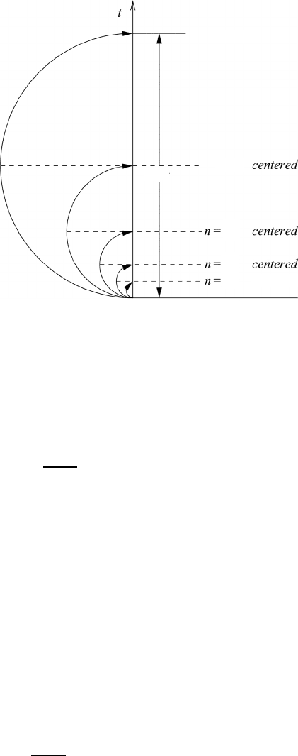
This suggests that we should use a combination of these two procedures, as will

be explained now. The numerical calculations are started by applying the forward-

in-time difference method for a fraction, say t



t, of the regular time step

t. In this way we calculate with a high degree of stability, without the presence

of the numerical wave, the variable ψ at the time t = t/8. In the second step

the normal solution scheme is applied, using the centered difference quotients with

t



t. In the third step one doubles the time step, i.e. t



t, thereby

always starting from n = 0. In the next step we use t



t until, in the

ﬁfth step with t



= t,thevalueofψ at time step n = 2 is obtained. The

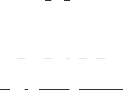
procedure, which is also known as the leap-frog method, is shown schematically

in Figure 25.3. By means of this successive initialization the phenomenon of the

weak instability is suppressed very efﬁciently. Much more could be said about this

and other calculation procedures, but we have given sufﬁcient evidence that great

care must be taken in applying ﬁnite-difference schemes. Later we will discuss an

entirely different instability, which is associated with the numerical treatment of

the nonlinear advection equation.

25.4 The implicit method

It is possible to give a numerical scheme for the solution of (25.1) that is abso-

lutely stable. In this case we proceed as follows. Time and spatial derivatives are

discretized by

∂ψ

∂t

n+1

− ψ

t

∂ψ

∂x



n+1

j+1

− ψ

n+1

j−1

2 x

j+1

− ψ

j−1

2 x



(25.38)

25.4 The implicit method 643

n = 1

forward

n = 2

2 ∆t

Fig. 25.3 The leap-frog method.

The partial derivative with respect to time is discretized by a forward-in-time

difference quotient while the partial spatial derivative is expressed by a mean value

in time. Therefore, the discretized form of equation (25.1) is given by

n+1

− ψ

Ut

4 x



n+1

j+1

− ψ

n+1

j−1

+ ψ

j+1

− ψ

j−1



= 0(25.39)

In contrast to the methods which we have discussed so far, the required grid function

at n + 1 now appears at three different places and cannot be determined explicitly

as before. Therefore, this difference method is called the implicit scheme.Inorder

to ﬁnd the solution of the advection problem, (25.39) must be written down for

all grid points j , including the boundary points j = 0andj = J . This leads to

a band matrix that can be solved by known methods for the required values ψ

n+1

with j = 1, 2,...,J − 1. We will not describe the numerical procedure, but the

numerical effort by far exceeds the computational labor of the explicit schemes.

This is the price to be paid for the stability of the numerical method.

In order to prove the stability of the scheme, we introduce the trial solution

(25.6a) into (25.39) and obtain

exp(−ikc t) − 1 +

Ut

4 x

[exp(ik x) − exp(−ik x)][exp(−ikc t) + 1] = 0

(25.40)

644 An excursion concerning numerical procedures

Dividing this equation by the expression within the second set of brackets gives

exp(−ikc t) − 1

exp(−ikc t) + 1

Ut

4 x

[exp(ik x) − exp(−ik x)] = 0(25.41)

On multiplying the numerator and denominator of the ﬁrst term by exp(ikc t/2)

and using well-known trigonometric relations we obtain without difﬁculty the

frequency equation

−i tan



kc t



+ i

Ut

2 x

sin(kx) = 0(25.42)

The required expression for the phase velocity follows immediately:

c =

kt

arctan



Ut

2 x

sin(kx)



(25.43a)

The argument of the arc tangent may become arbitrarily large since the tangent

may assume any value between minus and plus inﬁnity. This means that the phase

velocity is real for all values of t and x. For this reason the solution of the

difference equation (25.39) remains absolutely stable. Since arctan x ≈ x for

 1weﬁnd

lim

x,t→0

c = U (25.43b)

so that in the limiting case we obtain the required phase velocity.

The implicit method is used in many practical applications, since the CFL

criterion does not have to be obeyed in the implicit method. However, the smaller

the values of t and x the closer the agreement with the analytic solution, in

general.

The implicit treatment of the meteorological equations is very time-

consuming. In order to reduce the numerical effort Robert (1969) introduced the

so-called semi-implicit method. This is a procedure that treats implicitly only those

terms which are mainly responsible for the propagation of the high-speed waves

requiring very small time steps in the explicit treatment. The remaining terms are

treated explicitly. This leads to a considerable increase of t, which is now limited

only by the slower waves of meteorological signiﬁcance.

25.5 The aliasing error and nonlinear instability 645

25.5 The aliasing error and nonlinear instability

In order to demonstrate the existence of a different type of instability, we consider

the one-dimensional nonlinear advection equation

∂u

∂t

+ u

∂u

∂x

= 0(25.44)

which is always a part of the equations of motion. The analytic solution, as is easily

veriﬁed, is given by

u = f (x − ut)(25.45)

where f is an arbitrary function. We now consider the nonlinear term which results

from the multiplication of u and its spatial derivative. When the calculation is

performed in ﬁnite differences, we obtain an error due to the inability of the grid to

resolve wavelengths shorter than 2 x, or wavenumbers larger than k

max

= π/x.

Mesinger and Arakawa (1976) give an illuminating example by considering the

function

u = sin(kx)(25.46)

where k<k

max

. Substituting (25.46) into the nonlinear term gives

∂u

∂x

= k sin(kx)cos(kx) =

k sin(2kx)(25.47)

The wavenumber appearing in the sine wave of (25.47) is twice as large as the

original wavenumber in (25.46). Suppose that the wavenumber in (25.46) is in the

interval

max

<k≤ k

max

. It follows that the nonlinear term produces a wave that

cannot be resolved by the grid, which leads to an improper evaluation of the ﬁnite-

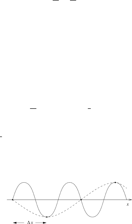
difference calculation. To gain further insight, consider a wave whose wavenumber

exceeds k

max

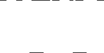
. This, for example, is the case if the wavelength is 4 x/3, as shown

by the full line in Figure 25.4.

Fig. 25.4 Misrepresentation of a wave of length 4 x/3 (full curve) as a wave of length

4 x due to the use of the ﬁnite-difference grid.

646 An excursion concerning numerical procedures

All we can know about a variable is its values at the grid points. Therefore, we

cannot distinguish this wave from the dashed-line wave of wavelength 4 x.This

misrepresentation is known as the aliasing error.

In the more general case the variable u will be represented by an inﬁnite series

of harmonic components of the type (25.46):

u =



with u

= sin(k

x)(25.48)

so that many nonlinear terms of the type sin(k

x)sin(k

x) will appear due to the

nonlinear term. This, of course, will falsify the energy spectrum of the process

to be studied. Since aliasing is due to nonlinear effects one speaks of nonlinear

instability. Apparently, this effect was ﬁrst encountered by Phillips (1956) in his

famous numerical experiment modeling the general circulation of the atmosphere.

Arakawa (1966) and Arakawa and Lamb (1977) constructed ﬁnite-difference

equations that suppress the effect of nonlinear instability by restricting the inter-

action between the resolved and unresolved scales. We refer to Kasahara (1977),

who used the simple nonlinear advection equation (25.44) to demonstrate the basic

property of the Arakawa scheme. First of all, we consider the integrated linear

momentum M

and the kinetic energy K

per unit mass



udx, K



dx (25.49)

The dependent variable u is deﬁned on a cyclic continuous domain from x = 0to

x = L so that u(0) = u(L). In the integrated form the advection equations for the

linear momentum and the kinetic energy can be written as

(a)



∂u

∂t

dx =−



∂u

∂x

dx =−



∂

∂x





dx = 0

(b)



∂

∂t





dx =−



∂

∂x





dx =−



∂

∂x





dx = 0

(25.50)

since u(0) = u(L). Equation (25.50a) implies the well-known space-centered

difference scheme

∂u

∂t

=−

j+1

)

− (u

j−1

)

4 x

(25.51)

Using (25.51), we may approximate (25.50a), to obtain

∂

∂t



j=1

=−

4 x



j=1

[(u

j+1

)

− (u

j−1

)

] = 0(25.52)

25.5 The aliasing error and nonlinear instability 647

where J = L/x must be a natural number. Hence it is seen that the ﬁnite-

difference scheme (25.51) conserves the momentum. It will be left as an excercise

to show that the kinetic energy is not conserved by using (25.51) as indicated by

∂

∂t



j=1

= 0(25.53)

The conservation of the momentum by itself does not ensure computational stabil-

ity.

Both momentum and energy may be conserved by using an alternate scheme.

By writing (25.44) in the form

∂u

∂t

=−u

∂u

∂x

=−



∂u

∂x

∂u

∂x



(25.54)

we ﬁnd the ﬁnite-difference approximation

∂u

∂t

=−



j+1

− u

j−1

2 x

j+1

)

− (u

j−1

)

2 x



(25.55)

It will be left as an exercise to show that the scheme (25.55) conserves the

momentum and the kinetic energy. A difference scheme may be stable if it conserves

both the momentum and the kinetic energy. Since no change in the potential energy

of the system occurs, the total energy is conserved. This prevents the spurious

growth of energy which may occur on using (25.51) and various other advection

schemes. Additional details are given by Washington and Parkinson (1986), where

further references may be found, particularly with respect to the use of spatial-

difference schemes.

It is well known that most numerical modeling of all scales of atmospheric ﬂow is

based on the approximation of horizontal derivatives by ﬁnite differences. The basic

concepts of ﬁnite-difference approximations are relatively simple to understand.

Indeed, much sophistication has gone into the construction of many ﬁnite-difference

schemes, which are needed in order to handle various ﬂow problems. It is fair to

say that numerical modeling of atmospheric ﬂow since the pioneering work by

Charney et al. (1950) has been a story of great success. Most of the numerical work

represents the meteorological variables in space and time on a ﬁnite-difference

grid. However, there are other methods for describing atmospheric ﬁelds. It has

been shown by various modelers of the atmospheric ﬂow that hemispheric and

global modeling can be advantageously carried out by means of a spectral model

that makes use of the orthogonality properties of the spherical functions. Various

versions of spectral models have been devised. In the next chapter we will brieﬂy

discuss the philosophy of the spectral model and show how the model equations

may be obtained.

648 An excursion concerning numerical procedures

25.6 Problems

25.1: Show that equation (25.39) can be expressed with the help of a band matrix

multiplying the vector



n+1

,ψ

n+1

,...



, where T denotes the transpose. The

boundary points are assumed to be independent of time; all ψ

are considered to

be known.

25.2: Show all steps between (25.41) and (25.43a).

25.3: Verify equation (25.53) by using equation (25.51).

25.4: Show that the momentum and the kinetic energy are conserved by using

(25.55).

Modeling of atmospheric ﬂow by spectral techniques

26.1 Introduction

The representation of atmospheric ﬂow ﬁelds by means of spherical functions has a

long history. Haurwitz (1940) represented the movement of Rossby waves by means

of spherical functions. The development of the spectral method for the numerical

integration of the equations of atmospheric motion goes back to Silberman (1954),

who integrated the barotropic vorticity equation in spherical geometry. The spectral

method attracted the attention of others and studies were performed, for example, by

Lorenz (1960), Platzman (1960), Kubota et al. (1961), Baer and Platzman (1961),

and Elsaesser (1966). Lorenz demonstrated that, for nondivergent barotropic ﬂow,

the truncated spectral equations have some important properties. Just like the exact

differential equations, they preserve the mean squared vorticity, called enstrophy,

and the mean kinetic energy. Platzman pointed out that this very desirable property

automatically eliminated nonlinear instability, which at that time was a substantial

difﬁculty in grid-point models. The early work made use of the so-called interaction

coefﬁcients to handle nonlinearity. This cumbersome procedure was replaced by the

efﬁcient transform technique for solving the spectral equations, which was devised

independently by Orszag (1970) and by Eliasen et al. (1970). In compressed form

the essential information on spectral modeling is given by Haltiner and Williams

(1980). Much valuable information about spectral techniques – which is usually

not readily available – can be extracted from the “gray” literature. We refer to an

excellent report by Eliasen et al. (1970). Finally, we refer the reader to an excellent

article on “Global modelling of atmospheric ﬂow by spectral methods”, by Bourke

et al. (1977). This article states the merits of the spectral relative to ﬁnite-difference

models. We will brieﬂy repeat these.

Foremost among the advantages of the spectral method relative to ﬁnite-

difference methods are

649

650 Modeling of atmospheric ﬂow by spectral techniques

(i) the intrinsic accuracy of evaluation of horizontal advection,

(ii) the elimination of aliasing arising from quadratic nonlinearity,

(iii) ease of modeling ﬂow over the entire globe, and

(iv) the ease of incorporation of semi-implicit integration over time.

These characteristics of the spectral method result in highly accurate and

stable numerics and efﬁcient and simple computer coding. The spectral transform

technique described in this chapter follows the description in Technical Report

No. 6 “The ECHAM 3 Atmospheric General Circulation Model”, DKRZ, Hamburg,

1993, where the operational forecast model is presented. The model equations are

based on various suitable approximations to simplify the required parameterizations

of ﬂuxes and the numerical procedures. These approximations include simpliﬁed

forms of the continuity equation and the heat equation. We do not discuss these

approximations but use the equations in the forms given in the previous chapters.

Since the model equations ignore the diffusion ﬂux of the dry air, it becomes

possible to reduce the system of continuity equations of the partial masses to a

single prediction equation for the moisture variable q = m

, which here refers

to the sum of the speciﬁc humidity for the vapor (m

), the speciﬁc liquid (m

), and

the speciﬁc ice content (m

). All physical effects are thought to be described by the

symbol Q

. The moisture equation in the model is structured in such a way that it

is compatible with the heat equation.

26.2 The basic equations

In this section we will present the basic equations used for the spectral representa-

tion. These are the horizontal equations of motion, the continuity equation and the

hydrostatic equation, the prognostic equations for temperature, and the moisture

variable q. These equations have been derived in previous chapters but need to be

rewritten to a certain extent. First of all we repeat the equation for the individual

derivative in the spherical system, see equation (19.15),

∂

∂t

a cos ϕ

∂

∂λ

∂

∂ϕ

∂

∂ξ

(26.1)

where we have used the unspeciﬁed general vertical coordinate ξ and r has been

replaced by the constant earth radius a. Robert (1966) has pointed out that it is

appropriate for the spectral representation of the ﬂow ﬁeld on the globe to replace

the original velocity components by the transformation

u =

cos ϕ

,v=

cos ϕ

(26.2)

For notational convenience it is costumary to introduce the symbol µ = cos θ =

sin ϕ,whereθ = π/2 − ϕ is the co-latitude. From this deﬁnition follows a