Zdunkowski W., Bott A. Dynamics of the atmosphere: A course in theoretical meteorology

Подождите немного. Документ загружается.

10.6 Problems 301

10.6 Problems

10.1: Find equation (10.63) from equation (10.55).

10.2: Verify all parts of equation (10.69).

10.3: Verify all parts of equation (10.72) by using the approximations which were

introduced just before this equation.

10.4: By utilizing the proper transformation rules given in Chapter M4 together

with the hydrostatic approximation, prove the validity of (10.75).

10.5: Start with equation (10.84) to verify the mathematical steps leading to

equation (10.93).

10.6: Verify equation (10.114).

Hint: Rewrite the right-hand side of equation (M6.49) in the form



L(t)

dr ·



∂A

∂t

− v ×∇×A



10.7: Apply the barotropic condition to show that

α ∇p =∇P

∗

with P

∗



αdp

∗

is a scalar ﬁeld function with P

∗

= 0atp = p

10.8: Derive equation (10.145) from equation (10.111).

Turbulent systems

The basic equations of motion and the budget equations presented so far refer to

the molecular system implying laminar ﬂow. The atmosphere, however, does not

behave like a laminar ﬂuid since it is turbulent everywhere and at all times. There-

fore, the pertinent equations have to be modiﬁed in order to handle turbulent ﬂow.

Since most meteorological observations represent average values over some time

interval and spatial region it will be necessary to average the governing equations of

the molecular system. In the next few sections some averaging procedures will be

discussed and averaging operators will be introduced. This leads to the introduction

of the so-called microturbulent system.

11.1 Simple averages and ﬂuctuations

There are several types of averages. Perhaps the best known average is the so-called

ensemble average, also known as the simple mean value or the expectation value.

For the arbitrary variable f the ensemble average is deﬁned by

f =



i=1

(11.1)

where the simple averaging operator is denoted by the overbar. Each of the f

represents one of N data points. We think of the ensemble as a large number of

realizations of a physical experiment carried out under identical external condi-

tions. The essential idea involved in the deﬁnition of the ensemble average is that

each individual realization f

is inﬂuenced by random errors that cannot be con-

trolled externally. In general, individual measurements will differ due to stochastic

disturbances.

We will now give some rules pertaining to the simple mean value. We deﬁne an

α quantity as a quantity that is the same for each member of the ensemble, meaning

302

11.1 Simple averages and ﬂuctuations 303

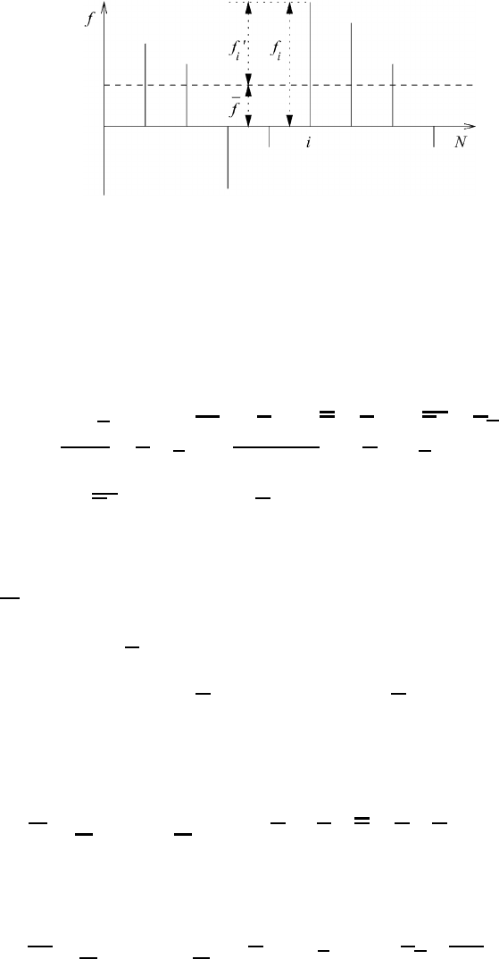
Fig. 11.1 A schematic representation of the ﬂuctuations and the mean value.

that α is independent of the subscript i,sothatα

= α. Obviously, the α quantity

includes all constants. Moreover, explicit functions of space and time, such as the

metric fundamental quantities, will not be averaged in the sense of (11.1). This

yields the following averaging rules:

α = α, αf = αf, f = f, fg = f g

f + g = f + g, α

f + α

g = α

f + α

(11.2)

In the expression fgthe average value f is common to all members of the ensemble.

Therefore, it is an α quantity and may be factored out of the sum. Repeated

averaging of a quantity that has already been averaged does not change its value.

This is known as the idempotent rule. The sum rules given in (11.2) demonstrate

that (

) is a linear operator.

The value f

of an ensemble will now be split into two parts. The deviation f



from the mean value f is known as the simple ﬂuctuation, as indicated in

= f + f



or f



= f

− f (11.3)

and depicted in Figure 11.1. From this expression it is easily seen that the average

value of the ﬂuctuations of the ensemble is zero:





i=1





i=1

− f ) = f − f = f − f = 0(11.4)

Of particular interest is the average of the product of two variables f and g:

fg =



i=1



i=1

(f + f



)(g + g



) = f g + f



(11.5)

304 Turbulent systems

since fg



= f g



= 0andf



g = f



g = 0. In this expression the so-called

correlation product



has been introduced according to





i=1



(11.6)

By utilizing the averaging rules (11.2) and (11.4) it is easily seen that the correlation

product can be written in various ways:



= f



g = fg



(11.7)

Let

δ represent a differential operator that is required to be the same for all

members of the ensemble so that δ is independent of the subscript i.Letthe

differential operator be applied to the variable f . Then the mean or average value

of this expression is given by

δf =



i=1

(δf )



i=1

= δf (11.8)

Since

δ is free from the subscript i we ﬁnd the interesting rule that the differ-

ential operator can be separated from the averaging operator (

). Examples are

δ = ∂/∂x,∂/∂t, ∇, etc. However, the budget operator δ = D/Dt as well as the

individual time derivative δ = d/dt do not follow this rule. Explicit expressions

for the budget operator and the total time derivative will be worked out later.

11.2 Weighted averages and ﬂuctuations

An important generalization of the simple mean value is the weighted mean value

or weighted expectation value deﬁned by



f =



i=1



i=1

(11.9)

The symbol



deﬁnes the weighted-averaging operator. The various ρ

are the

weights. From (11.1) and (11.9) it follows that



f =

ρf

=⇒ ρf = ρ



(11.10)

11.2 Weighted averages and ﬂuctuations 305

which is also known as the Hesselberg average. Equations (11.9) and (11.10) will

be used many times in the following sections.

Some of the rules given for the simple average are of general character and,

therefore, may also be applied to the weighted average. In analogy to (11.2) the

weighted average is independent of the subscript i so that it can be handled as an α

quantity. Furthermore, the sum rules also apply to the weighted average, yielding

α = α,



αf = α



f =







fg =



f g

(f + g) =



f +g, (α

f + α

g) = α



f + α

g

(11.11)

Thus, the weighted average also has the properties of a linear operator. Additional

rules are given in



fg = fg,



f = f,



f =



f (11.12)

These are largely self-explanatory.

Let us again consider the differential operator

δ applied to the variable f .The

weighted average of this expression is given in



δf =



i=1

(δf )



i=1

= δ



f since



f =





i=1

(ρ

)



i=1



(11.13)

Thus, in contrast to (11.8), which refers to the simple mean, it is not possible to

separate

δ from the weighted average.

In analogy to (11.3) we now split the variable f into its weighted mean



f and

ﬂuctuation f





f + f



or f



= f

−



f (11.14)

whereby the mean or average value of the weighted ﬂuctuation also vanishes:







i=1





i=1



i=1

−



f )



i=1



f −



f = 0(11.15)

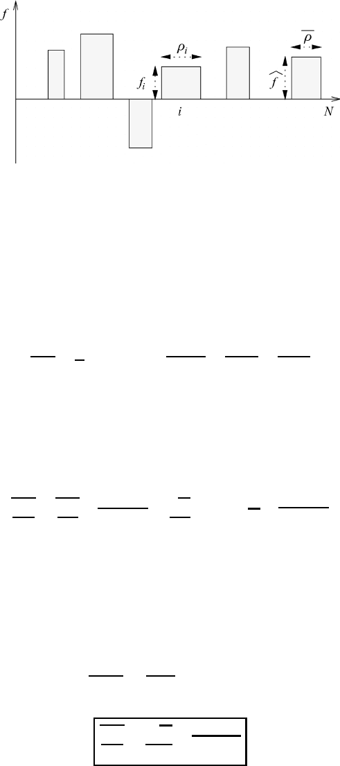
In order to get a clearer picture of the meaning of the weighted average, let us

consider Figure 11.2. We observe that each member of the ensemble is characterized

by a rectangular area of height f

and width ρ

. The rectangular area on the right-

hand side of Figure 11.2 represents the average area F = ρf = ρ



f . The height of

this rectangular area is the weighted value



f while the width is given by ρ.

Mean values of ﬂuctuations vanish only if ﬂuctuations and the type of the average

correspond, as demonstrated in



= f −



f =

f −



f = 0,







f −



f =



f − f = 0

(11.16)

306 Turbulent systems

Fig. 11.2 A representation of the weighted average and the weights.

The product rule



fg =



fg +





(11.17)

corresponds fully to (11.5). The correlation





may be written in various ways

as shown in









g =





(11.18)

This property turns out to be very helpful, as will become apparent in later sections.

Other important relations following from (11.10) and (11.18) are

ρf



= ρ





= 0, ρf



= ρf



g = ρf g



(11.19)

11.3 Averaging the individual time derivative and the budget operator

As has already been mentioned, great care must be taken when one is averaging

the individual time derivative d/dt and the budget operator D/Dt.Wewillnow

show how to proceed. The ﬁrst step for the individual time derivative is given by

dψ

∂ψ

∂t

·∇ψ =

∂ψ

∂t



·∇ψ + v



·∇ψ (11.20)

Here the velocity vector v

has been split into its weighted average



,which

is treated as an α quantity, and the ﬂuctuation v



. Utilizing a rigidly rotating

coordinate system with v

= 0, we have v

= v + v



and v



= v



since v



an explicit function of space. Recall that, according to (11.8), ∂/∂t and ∇ may

be separated from the simple average operator. By deﬁning the individual time

derivative of the averaged system by means of



d ...

∂...

∂t



·∇... (11.21)

we ﬁnally obtain for the averaged individual time derivative

dψ



+ v



·∇ψ

(11.22)

11.4 Integral means 307

In complete analogy we proceed with the budget operator and obtain

(ρψ) =

∂

∂t

(

ρψ) +∇·(



ρψ) +∇·(v



ρψ)



(

ρψ) +∇·v



ρψ

with



D...

∂...

∂t

+∇·(



...)

(11.23)

Averaging the molecular form of the continuity equation yields the expression

∂ρ

∂t

+∇·(ρv

) =

∂

∂t

+∇·(



ρ) =



ρ = 0

(11.24)

where we have used the Hesselberg averaging procedure. Here the advantage of

the Hesselberg mean becomes clearly apparent since the averaged form of the

continuity equation (11.24) is completely analogous to the molecular form. Had

we used the Reynolds mean then the additional term

∇·v



, which is not easily

accessible, would have appeared in the averaged continuity equation.

In the exercises we will show that the interchange rule (M6.68) of the molecular

system also holds for the averaged system



(

ρψ) = ρ



dψ

(11.25)

11.4 Integral means

Obviously, we are unable to control the atmosphere so that it is impossible to

produce and observe identical weather systems. Therefore, the ensemble average is

of doubtful practical use. For this reason we direct our attention to time and space

averages. The time average at a ﬁxed point is deﬁned by means of

(r,t) =

t



t+t/2

t−t/2

ψ(r,t,t



) dt



(11.26)

where t is a suitable averaging interval about t and ψ is the quantity to be

averaged over time at the ﬁxed position r. The integral mean can be obtained for

the Cartesian system as well as for the general q

system by using the proper metric

fundamental quantities. To give a speciﬁc example, let us consider the hypothetical

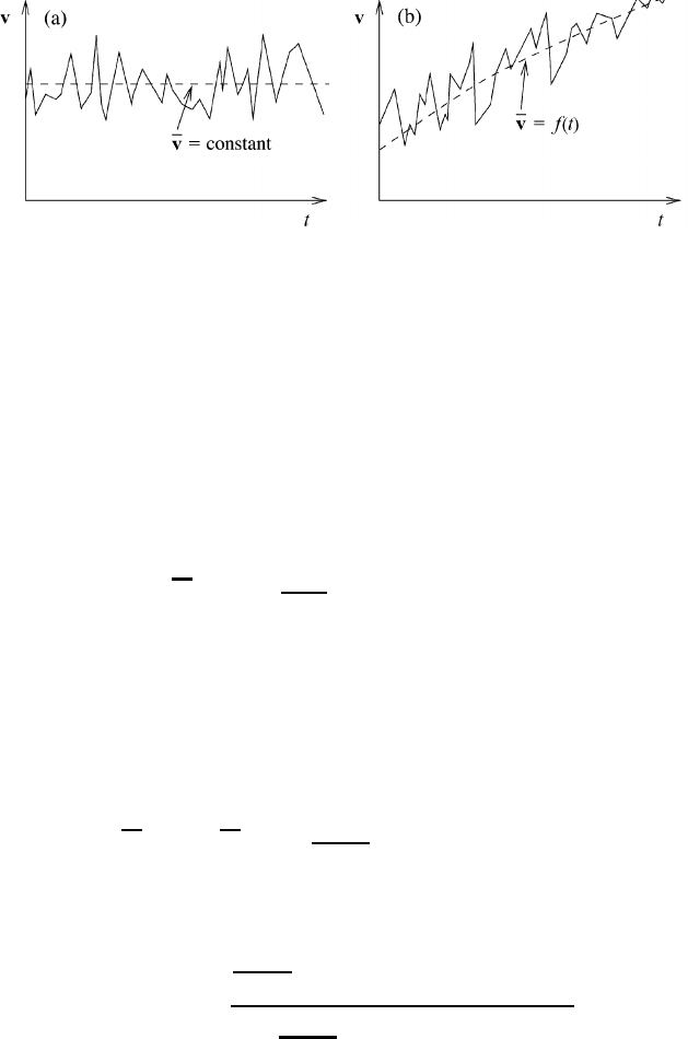
velocity spectrum shown in Figure 11.3. For turbulent steady ﬂow the average

308 Turbulent systems

Fig. 11.3 (a) Turbulent steady ﬂow. (b) Turbulent unsteady ﬂow.

is time-independent; see Figure 11.3(a). For extended time intervals the average

itself may become a function of time, as shown in part (b) of Figure 11.3. The

time-dependent mean is often called the gliding mean or the moving mean.

According to the choice of the averaging interval, the gliding mean has the

tendency to suppress a part of the high-frequency ﬂuctuations. For this reason the

gliding mean acts as a low-pass ﬁlter. In the same sense most measuring devices

act as low-pass ﬁlters since they are incapable of recording rapid oscillations.

Next we deﬁne the spatial mean for ﬁxed time by

(r,t) =

V (r)



V (r)

ψ(r, r



,t) dV



(11.27)

There is a problem with this type of mean since we generally cannot expect that

the value measured at a certain point is representative of a larger surrounding area.

Since the observational grid is rarely dense enough to evaluate (11.27), we are

hardly able to use this equation. For our purposes, however, it seems convenient to

think of the average as a space-time average deﬁned either by

ψ(r,t) = ψ(r

) =

G(r

)



G(r

)

ψ(r

, r



) dG



(11.28)

or by



ψ(r,t) =



ψ(r

) =

G(r

)



G(r

)

ρ(r

, r



)ψ(r

, r



) dG



G(r

)



G(r

)

ρ(r

, r



) dG



(11.29)

representing the simple and weighted means. Here we have formally introduced the

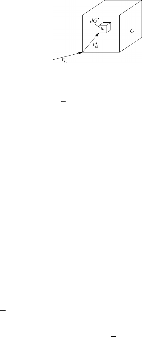
space-time vectors r

and r



as shown in Figure 11.4. Actually space-time vectors

cannot be made visible, but this ﬁgure is a good tool for demonstration purposes. r

is the space-time vector of the original system whereas r



is the space-time vector of

11.4 Integral means 309

Fig. 11.4 Averaging for ﬁxed r and t (i.e. r

= constant) over the space-time ‘volume’ G.

the averaging space-time ‘volume’ G whose origin is taken at the endpoint of r

.For

the Cartesian system we have dG



= dG



= dx



whereas for the general

system dG



= dG



√



. During the averaging process the

space-time volume G and r

are ﬁxed while the averaging itself is carried out with

the help of r



so that the coordinates of r

and r



are entirely independent.

Let us now consider the special situation that the statistical parameters charac-

terizing the turbulence are independent of space and statistically not changing with

time. In this case we speak of homogeneous and stationary turbulence.Nowthe

ensemble, time, and space averages yield the same results. This is known as the

ergodic condition. To make the turbulence problem more tractable, in our studies

we will assume that the ergodic condition applies. Thus, all results obtained with

the help of the ensemble average will be considered valid for the other averages as

well.

To get a better understanding of the concept of averaging, we will show how

the one-dimensional ensemble average can be transformed into the corresponding

integral average if the number of realizations N becomes very large. Moreover,

we will demonstrate with the help of Figure 11.5 how to usefully interpret the

average and what is meant by holding x constant and by the integration over x



.Let

us consider the hypothetical spectrum depicted in Figure 11.5(a). First we select

the averaging interval x which is centered at x

. Then we rotate the averaging

interval by 90

◦

at the point x

and introduce the x



-axis as shown in part (b) of

Figure 11.5. At the point x

one now has a collection of N realizations x



, implying

N ﬂuctuations.

On integrating over this newly formed collection of N realizations we ﬁnd at the

point x

the ensemble average, which transforms to the integral average:

) = lim

N→∞





j=1

ψ(x



)



x



+x/2

−x/2

ψ(x



) dx



(11.30)

if N becomes very large. The rotation is then carried out at each point of the x-axis

so that for each x value one has a mean value

ψ(x) representing N ﬂuctuations.

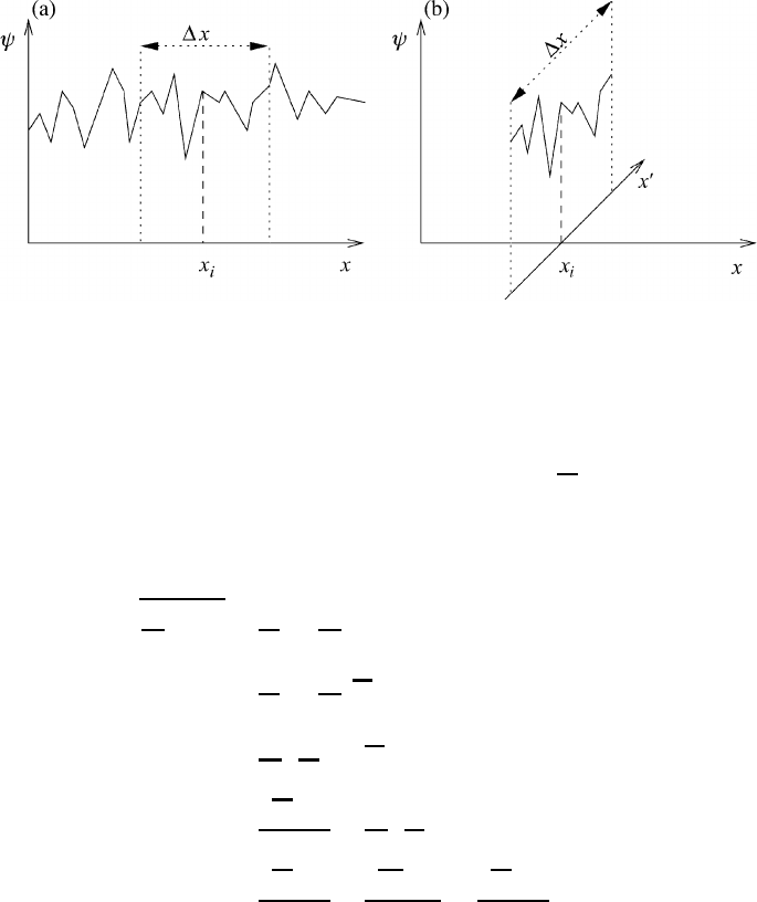
310 Turbulent systems

Fig. 11.5 A schematic representation

of the averaging procedure for a one-dimensional

spectrum.

In another example we are going to show that the derivative of the time average

as found from the deﬁnition of the ensemble average may also be found from the

integral deﬁnition. By observing that the average quantity

ψ depends only on r

and not on r



and that the boundaries of the averaging domain G are held ﬁxed,

we obtain according to the Leibniz rule

∂

∂t

ψ(r

) =



∂

∂t

ψ(r

, r



) dG





∂

∂t



ψ(r

) + ψ



, r



)





∂

∂t







ψ(r

) + ψ



, r



)







∂

ψ(r

)

∂t

∂

∂t







, r



) dG





∂

ψ(r

)

∂t

∂



)

∂t

∂

ψ(r

)

∂t

(11.31)

The last integral in (11.31) represents the mean value of the ﬂuctuations and must

vanish. Analogous arguments hold for the space derivatives.

11.5 Budget equations of the turbulent system

As we have pointed out several times, each of the important atmospheric prog-

nostic equations of the molecular system can be written in the form of the

budget equation. We will now proceed and derive the general form of the bud-

get equation for the microturbulent system, which for simplicity will henceforth