Webster R., Oliver M.A., Geostatistics for Environmental Scientists

Подождите немного. Документ загружается.

4.9.3 Average semivariances

If we recall the deﬁnition of the semivariance from equation (4.13) as

gðhÞ¼

E fZðxÞZðx þ hÞg

ð4:38Þ

then its estimator is

gðhÞ¼

mean fzðxÞzðx þ hÞg

; ð4:39Þ

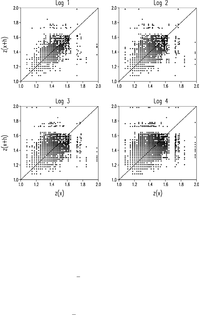
Figure 4.9 The h-scattergrams for four lags computed from the data of log

Kat

Broom’s Barn Farm.

Estimating Semivariances and Covariances 67

where the zðxÞ and zðx þ hÞ represent actual values of Z at places separated by

h. For a set of data zðx

Þ; i ¼ 1; 2; ...; we can compute

gðhÞ¼

2mðhÞ

mðhÞ

i¼1

fzðx

Þzðx

þ hÞg

; ð4:40Þ

where mðhÞ is the number of pairs of data points separated by the particular lag

vector h. By changing h we obtain an ordered set of semivariances, which

constitute the experimental variogram or sample variogram. Equation (4.39) is the

usual formula for computing semivariances; it is commonly known as

Matheron’s method-of-moments estimator. The way that it is implemented as

an algorithm depends on the conﬁguration of the data, and we consider the

possibilities below.

Regular sampling in one dimen sion

For regular sampling in one dimension along transects and down boreholes we

can den ote the data by z

¼ zðx

Þ; i ¼ 1; 2; ...; N. The lag becomes a scalar,

h ¼jhj, for which

g can be computed only at integral multiples of the sampling

interval. The semivariance is then computed as

gðhÞ¼

2ðN  hÞ

Nh

i¼1

 z

iþh

: ð4:41Þ

Figure 4.10(a) shows the situation. First, the squared differences between

neighbouring pairs of values, z

and z

, z

and z

, and so on, i.e. for h ¼ 1, are

determined for each position and averaged. All of the observations at lag interval

h are used twice except for those at the ends of the transect, and so there are N  1

comparisons. If there are missing values at some locations, as in Figure 4.10(b),

then there will be fewer comparisons, and the divisor is diminished accordingly.

By increasing h to 2 the comparisons are then z

with z

, z

with z

, etc., and we

can repeat the procedure for h ¼ 3; 4; ... . The result is a set of semivariances

gð1Þ;

gð2Þ;

gð3Þ; ... that is ordered as a function of h. It is a one-dimensional

experimental variogram, and we can plot

gðhÞ against h as in Figure 4.11.

Irregular sampling in one dimension

If data are irregularly scattered then the average semivariance for any

particular lag can be derived only by grouping the individual lag distances

between pairs of points into ‘bins’ as in a histogram. Otherwise we have

individual semivariances as in the variogram cloud. Typically the averaging

is done by choosing a set of lags, h

; j ¼ 1; 2; ...; at arbitrary constant

increments d, and then associating with each h

a bin of width d, bounded by

 d=2 and h

þ d=2. Each pair of points separated by h

 d=2 is used to

estimate gðh

Þ. In this way each comparison contributes to one and only one

68 Characterizing Spatial Processes

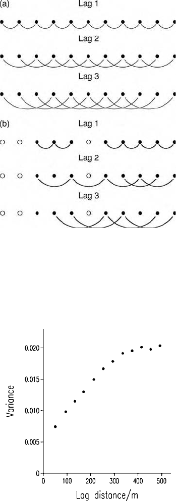
Figure 4.10 Comparisons for computing a variogram from regular sampling on a

transect: (a) with a complete set of data, indicated with ; (b) with missing values,

indicated by .

Figure 4.11 Sample variogram of log

K at Broom’s Barn, obtained by discretization

of the lags into bins as in Figure 4.13.

Estimating Semivariances and Covariances 69

estimate. Sometimes there are more comparisons at the shorter lags, especially

where sampling has been nested (see Chapter 6), and then it can be advanta-

geous to increase the increments, and with them d,ash increases.

The lag increments can affect the resulting variogram, and so d should be

chosen with care. If the increment is small then there might be too few

comparisons at each lag, leading to semivariances that are estimated crudely

and an experimental variogram that appears erratic. If, on the other hand, d is

large then there are likely to be few estimat es and detail is lost by unnecessary

smoothing. The best compromise will depe nd on the number of data, the

evenness of the sampling and the form of the underlying variogram. A useful

starting point is to use the average separation between nearest neighbours as

the interval.

Sampling on transects to represent variation in two dimensions

Sometimes investigators sample regularly along tran sects to explore variation

in two dimensions and, in particular, to identif y and estimate anisotropy, i.e.

directional differences. The computational procedure is the same as for the

regular one-dimensional sampling, and equation (4.41) produces a separate set

of estimates for each transect. These need to be seen together as a whole and

not as separate variograms. The variogram in two dimensions is itself two-

dimensional, and the ordered sets of semivariances computed from transects are

effectively samples of sections through the two-dimensional function. To

identify and estimate ani sotropy, transects must be aligned in at least three

directions. If the directional variogram appears to have markedly different

gradients or ranges in the different directions then it is likely that the under-

lying variation is anisotropic, and it should be modelled accordingly (see

Chapter 5). If the variation seems isotropic, i.e. if there are no directional

differences, then the separate estimates can be averaged over all directions to

give the isotropic variogram where the vector h can be replaced by the scalar

h ¼jhj.

Regular sampling in two dimensions

For data recorded at regular intervals on a rectangular grid the above formula

(4.41), for one dim ension, is readily extended. If the grid has m rows and n

columns then we compute

gðp; qÞ¼

2ðm  pÞðn  qÞ

mp

i¼1

nq

j¼1

fzði; jÞzði þ p; j þ qÞg

;

gðp; qÞ¼

2ðm  pÞðn  qÞ

mp

i¼1

nq

j¼qþ1

fzði; jÞzði þ p ; j  qÞg

;

ð4:42Þ

70 Characterizing Spatial Processes

where p and q are the lags along the rows and down the columns of the grid,

respectively. In general, the lag increment is simply the grid interval. These

equations enable hal f the variogram to be computed for lags from q to q and

from 0 to p. The variogram is symmetrical about its centre, and the full set of

semivariances is obtained by computing

gðp; qÞ¼

gðp; qÞ;

gðp; qÞ¼

gðp; qÞ:

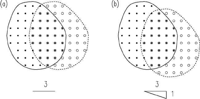
The procedure can be envisaged as moving the grid over itself to the right

and up or down to new positions, as in Figure 4.12, and making the

comparisons between the values at the points that coincide. In Figure 4.12(a)

the grid has been moved to the right by three units, i.e. p ¼ 3 and q ¼ 0, as

represented by the horizontal line. In Figure 4.12(b) the grid has been moved

down one unit in addition, so that now q ¼1; the horizontal and

vertical shifts are shown in the triangle, with its hypotenuse showing the

resultant.

Figure 4.12 also shows that as p and q are increased so the number of

coincident points diminishes rapidly from the original 55. As a consquence the

semivariances become less and less well estimated, a matter to which we return

in Chapter 6.

Where data are missing, the quantities (m  p)(n  q) in the denominators of

equation (4.42) mu st be replaced by the actual numbers of comparisons.

Figure 4.12 Computing a two-dimensional variogram from a regular grid of data by

sliding the grid over itself: (a) by three units to the right; (b) by one unit down in

addition, with resultant lag given by the hypotenuse of the triangle.

Estimating Semivariances and Covariances 71

Irregular sampling in two dimensions

Survey data in two dimensions are often unevenly distributed. Each pair of

observations is separated by a potentially unique lag in both distance and

direction. To obtain averages containing directional information we must group

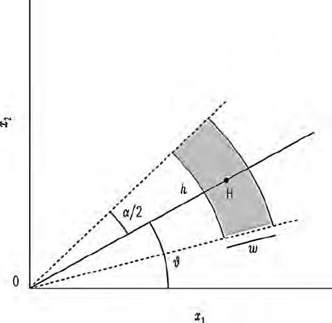
the separations by direction as well as by distance. Figure 4.13 shows the

geometry of the grouping. We choose a lag interval, the multiples of which will

form a regular progression of nominal lag distances as in the one-dimensional

case. We then choose a range in distance, w in Figure 4.13, usually equal to the

lag interval. The nominal lag distance is represented by the line OH of length h.

We also choose a set of directions, one of which is shown as # in Figure 4.13, and

a range in direction, a, such that a ¼ p=n, where n is the number of directions,

and # progresses in steps of a from 0 to p=ðn  1Þ. For example, if we choose four

directions ðn ¼ 4) then a sensible progression for # would be 0, p=4, p=2, 3p=4,

i.e. 0, 45, 90, 135 degrees, with a ¼ p=4(45



). This ensures complete coverage

and no overlap between the different directions. For six directions a would be 30



Then for a point x

at O with a second point x

þ h within the stippled zone

fzðx

Þzðx

þ hÞg

contributes to

gðhÞ¼

gðh;#Þ. When all comparisons have

been made the experimental variogram will consist of the set of averages for the

nominal lags in both distance and direction. We can extend this further by

Figure 4.13 The geometry for discretizing the lag into bins by distance and direction in

two dimensions.

72 Characterizing Spatial Processes

computing the average experimental variogram over all directions (ominidirec-

tional) by setting a ¼ p (180



). Appendix B gives the GenStat instructions for

computing directional and omnidirectional variograms.

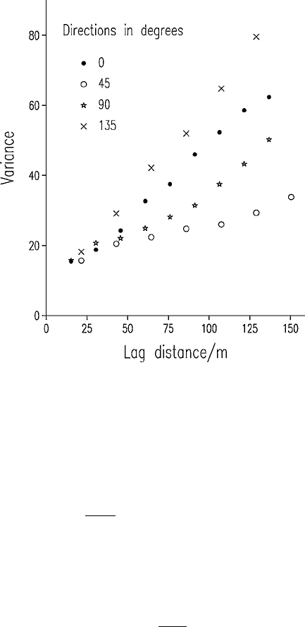
Exploring and displaying anisotropy

So far we have concentrated on explaining the computation in one and two

dimensions, but there is also the matter of repr esenting the results of the two

spatial dimensions on a plane, and of exploring differences in the variation in

two dimensions.

Where data are on a rectangular grid we can plot the semivariances along

the rows and columns and tho se on the principal diagonals separately, bearing

in mind that the lag intervals will not be the same in all four directions. No

directional information is lost, and the results can then be examined for

directional differences. Where data are irregularly scattered and we have to

group the angular separations then we inevitably lose some of the directional

information. The wider is a the more information we lose, until when a ¼ p

(180



) all is lost. Choosing a is therefore a compromise between a stable

estimate based on many comparisons over a wide angle that will underestimate

variance in the direction of the maximum and overestimate that in the direction

of the minimum, and one that is subject to large error but which gets closer to

the true values in the directions of maximum and minimum. At the outset a

reasonable rule of thumb is to let a ¼ p=4. If this appears to reveal anisotropy

then try reducing a until the resulting variogram becomes too erratic. The

larger is a, the more the anisotropy ratio will be underestimated when models

are ﬁtted (see Chapter 6). If the variation is isotropic the vector h can be

replaced by the scalar h ¼jhj in distance only, and the general computing

formula, equation (4.40), can be used. In this case we set a ¼ p to compute the

omnidirectional variogram.

Whereas it is easy to draw and comprehend a graph of the experimental

variogram for either one-dimensional data or one averaged over all directions in

two dimensions, it is much less so for the two-dimensional experimental

variogram. One simple way is to plot the values with a unique symbol for

each direction on the same pair of axes (Figure 4.14). Alternatively, some kind

of statistical surface can be ﬁtted to the two-dimensional variogram to represent

it as an isarithmic chart or perspective diagram (Figures 4.15 and 4.16). When

the variogram has been modelled, this surface can be that of the model. The

ideal solution would be to draw it as a stereogram.

4.9.4 The experimental covariance function

All of the above considerations also apply to the estimation of spatial covar-

iances, and the equations are analogous. Remember, however, that the

Estimating Semivariances and Covariances 73

covariance requires stationarity of the mean and the variance of the underlying

process. The general computing formula for the experimental covariance at lag

h, the analogue of equation (4.40), is

CðhÞ¼

mðhÞ

i¼1

fzðx

Þzðx

þ hÞg 



; ð4:43Þ

where



z is the mean of all the data. The analogous correlation function, the

sample correlogram, is readily derived from

CðhÞ by

rðhÞ¼

CðhÞ

; ð4:44Þ

where s

is the variance of the data.

If ZðxÞ is second-order stationary then

CðhÞ

Cð0Þ

gðhÞ for all h. If there

is trend in the variation then

Cð0Þ

gðhÞ will tend to be larger than

CðhÞ

computed by equation (4.43). This tendency can be counteracted by replacing

the regional mean



z by two distinct means, one the mean of the

Figure 4.14 A two-dimensional variogram with a distinct symbol for each of four

directions.

74 Characterizing Spatial Processes

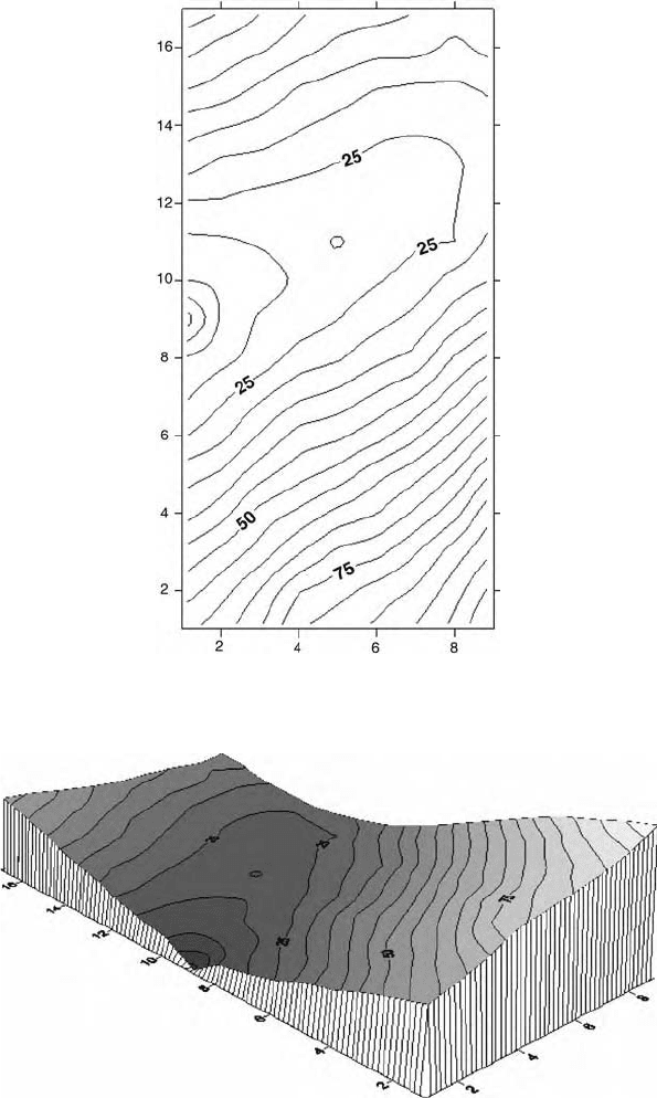
Figure 4.15 An isarithmic chart of a two-dimensional variogram. The origin is in the

middle of the left-hand side.

Figure 4.16 A persective diagram of a two-dimensional variogram. The origin is in the

middle at the left front.

Estimating Semivariances and Covariances 75

zðx

Þ; i ¼ 1; 2; ..., say



, and the other the mean of the zðx

þ hÞ,



, and

computing

CðhÞ¼

mðhÞ

i¼1

fzðx

Þ



gfzðx

þ hÞ



g: ð4:45Þ

This measure of the covariance corresponds with that often used in statistics.

We no longer assume implicitly that



is the same as



. Several spatial

analysts, e.g. Deutsch and Journel (1992) and Isaaks and Srivastava (1989),

use this formula as a matter of course. They call the quantities



and



the

means of the ‘heads’ and of the ‘tails’, respectively.

Similarly the autocorrelation coefﬁcients can be estimated by

rðhÞ¼

CðhÞ

; ð4:46Þ

where s

and s

are the standard deviations of the heads and tails. These

formulae are used by time-series analysts, but Yule and Kendall (1950) warn

against using equation (4.46) if you have rather few data.

76 Characterizing Spatial Processes