Webster R., Oliver M.A., Geostatistics for Environmental Scientists

Подождите немного. Документ загружается.

Characterizing Spatial

Processes: The Covariance

and Variogram

4.1 INTRODUCTION

The previous chapter describes several of the common methods of spatial

interpolation. Some of them are crude, so that maps made using them display

the spatial variation poorly. The interpolators also fail to provide any estimates

of the error, which are desirable for prediction. The conventional approach to

spatial prediction in soil science combines classical estimation with spatial

classiﬁcation and thereby overcomes some of these weaknesses. It is the only

method described in Chapter 3 that gives sound estimates of error. However, it

requires replicated sampling for each class to provide individual estimates for

that class and some degree of randomization of the sam ple. The sampling effort

can be large, but even with such effort the predicted values at all points within a

given class are simply the mean of that class for the property of interest. The

precision of prediction is limited by the goodness of the classiﬁcation; variation

within classes is ignored, and local variation is not resolved.

Mathematical functions of the spatial coordinates seemed at one time to have

promise. They could be deﬁned fully, and they could therefore be used

repeatably. Most were also intuitively reasonable. Some, such as the inverse

functions of distance and triangulation, however, were also quite arbitrary,

taking no account of more general knowledge of the variation in the region.

Trend surface analysis, the only function described in Chapter 3 that does

recognize the generality, has other defects.

The methods are deterministic, and to that extent they accord with

our understanding that the variation in the environme nt has physical causes,

i.e. is physically determined. However, the environment and its component

attributes, such as the soil, result from many physical and biological processes

Geostatistics for Environmental Scientists/2nd Edition R. Webster and M.A. Oliver

# 2007 John Wiley & Sons, Ltd

that interact, some in highly non-linear and chaotic ways. The outcome is so

complex that the variation appears to be random. This complexity, together

with our current, far from complete, unders tanding of the processes, means that

mathematical functions are not adequate to describe any but the simplest

components.

A fully deterministic solution to our problems seems out of reach at present.

To make progress we must look at spatial variation differently. Recapitulating,

we have two needs: to describe quantitatively how soil varies spatially, and to

predict its values at places where we have not sampled. In addition we want

estimates of the errors on these predictions so that we can judge what

conﬁdence to place in them; estimates of errors are lacking in the classical

methods of interpolation. We need a model for prediction, and since there is no

deterministic one the solution seems to lie in a probabilistic or stochastic

approach.

4.2 A STOCHASTIC APPROACH TO SPATIAL VARIATION:

THE THEORY OF REGIONALIZED VARIABLES

4.2.1 Random variables

The fact that spatial variation appears to be random suggests a way forward.

Consider throwing a die; on any one throw we obtain a number, for instance, a

6. This is the outcome of throwing the die once, of drawing one value from a

distribution that consists of the set f1; 2; 3; 4; 5; 6g with equal probability. One

can argue that the result is physically determined in that it depends on the

position of the die in the cup and of the cup itself at the start, the forces imparted

to it by the thrower, and the nature of the surface on which it lands (Matheron,

1989). Nevertheless, these are so imperfectly known and so far beyond our

control that we regard the process as random and as unbiased. Similarly, since

the factors that determine the values of environmental variables are numerous,

largely unkno wn in detail, and interact with a complexity that we cannot

disentangle, we can regard their outcomes as random.

If we adopt a stochastic view then at each point in space there is not just one

value for a property but a whole set of values. We regard the observed value

there as one drawn at random according to some law, from some probability

distribution. This means that at each point in space there is variation, a concept

that has no place in classical estimation. Thus, at a point x a property, ZðxÞ,is

treated as a random variable with a mean, m, a variance, s

, and higher-order

moments, and a cumulative distribution function (cdf). It has a full probability

distribution, and it is from this that the actual value is drawn. If we know

approximately what that distribution might be we can estimate values at

unrecorded places from data in the neighbourhood and put errors on our

estimates.

48 Characterizing Spatial Processes

Most environmental variables, such as the soil’s pH and potassium concen-

tration, are continuou s. For these a value zðxÞ can be thought of as one of an

inﬁnite number of possible values, with a cdf that is the probability that Z takes

any valu e less than or equal to a particular value z

FfZðx; zÞg ¼ Prob½ZðxÞz

 for all z: ð4:1Þ

The probabilility FfZðx; zÞg takes values between 0 and 1. Its derivative is the

probability density function, the pdf:

f fZðxÞg ¼

dFfZðx; zÞg

; ð4:2Þ

which we described in Chapter 2. The distribution may be bounded, as in the

case of a proportion or percentage, but the most useful assumption is that it is

not, so that 1  ZðxÞþ1.

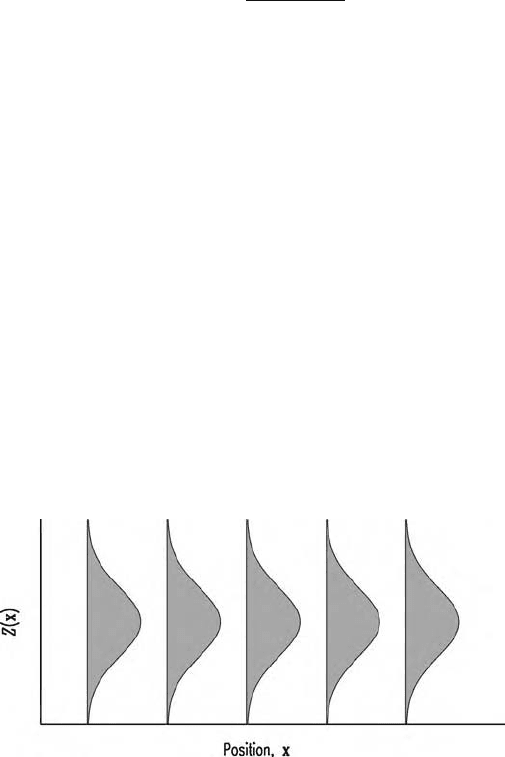
4.2.2 Random functions

The description above for an individual point x applies to the inﬁnitely many points

in the space; at each point x

; i ¼ 1; 2; ... , Zðx

Þ has its own distribution and cdf.

The range of possible values constitutes an ensemble, and one member of the

ensemble is the realization. The idea is illustrated in Figure 4.1 in which the curves

are imagined to protrude vertically out of the plane of the page. The set of random

variables, Zðx

Þ;Zðx

Þ; ...; constitute a random function,arandom process,ora

stochastic process. The set of actual values of Z that comprise the realization of the

random function is known as a regionalized variable. Just as in Chapter 2 we

regarded a region as made up of a population of units, so we can think of a random

function ZðxÞ as a superpopulation, with an inﬁnite number of units in space and

an inﬁnite number of values of Z at each point in the space. It is doubly inﬁnite.

Figure 4.1 The normal distributions of the random variables at ﬁve sites.

A Stochastic Approach to Spatial Variation 49

4.3 SPATIAL COVARIANCE

To deﬁne the variation we need to describe the ensemble simply. For the

possible outcomes of throwing the die it is easy because they are independent.

The values of regionalized variables, on the other hand, tend to be related. In

general, values at two places near to one ano ther are similar, whereas those at

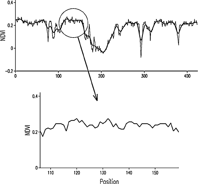
more widely separated places are less so. This can be seen in Figure 4.2, which

represents pixel values for the normalized difference vegetation index (NDVI),

where

NDVI ¼ðinfrared  redÞ = ðinfrared þ redÞ; ð4:3Þ

along one row of a SPOT (Syste`me Probatoire de l’Observation de la Terre)

image (fro m Oliver et al., 2000). The ﬁne line joining the pixel values in the

Figure 4.2 Transect across a SPOT image for normalized difference vegetation index.

The ﬁne line in the upper graph joins the data, and the bold line is a smoothing spline

ﬁtted through them. The lower graph is an enlarged version of the section in the circle.

50 Characterizing Spatial Processes

upper graph illustrates the locally erratic nature of the variation. Wherever

we look we see some ﬂuctuation, but in most short sections of the transect the

values are similar. Over longer distances, however, the values vary more

substantially, with some sections having small values on average and others

where they are large. This becomes clear when the locally erratic variation has

been ﬁltered by a smoothing spline, the bold line in the grap h. Where the

property is continuous, as in this example and as is the case for most properties

of the environment, its values must be related at some scale. This is illustrated

further in the lower graph where a small section of the transect is magniﬁed

and the pixel values are plotted in more detail. What appeared to be entirely

erratic in the upper graph can be seen at the larger resolution as structured in

the sense that neighbouring values are similar to one another on average. We

want to describe these relations, and we do so using the concept of covariance.

We are likely to be fam iliar with using the covariance to determine

the relation between two variables for paired observations. For n pairs of

observations, z

i;1

; z

i;2

; i ¼ 1; 2; ...; n, of two variables, z

and z

, the covariance

is given by

Cðz

; z

Þ¼

i¼1

i;1





gfz

i;2





g; ð4:4Þ

where



and



are the means of z

and z

, respectively. If the units,

i ¼ 1; 2; ...; n, on which the observations were made were drawn at random

then

Cðz

; z

Þ estimates the population covariance without bias.

We can extend this deﬁniti on for relating two random variables. The concept

and its mathematical expression were developed originally for analysing time

series during the 1920s and 1930s, and they have been much used for

processing signals and for forecasting. They are now described in many text-

books, of which we can recommend Jenkins and Watts (1968) and Priestley

(1981). They have their analogies in space, and Yaglom (1987) presents them

in this context as underpinning spatial prediction.

In our new spatial setting z

and z

become Zðx

Þ and Zðx

Þ, i.e. they are the

sets of values of the same property, Z, at the two places x

and x

, and we have

switched the notation to capital Z to signify that they are random variables.

Their covariance is

Cðx

; x

Þ¼E½fZðx

Þmðx

ÞgfZðx

Þmðx

Þg; ð4:5Þ

where mðx

Þ and mðx

Þ are the means of Z at x

and x

. The equation is

analogous to equation (4.4). Unfortunately, however, its solution is unavailable

because we have only the one realization of Z at each point; we cannot know the

means. Thus we seem to have reached an impasse, and we can progress only by

making further assumptions of stationarity which allow us to treat the values at

different places as though they are different realizations of the property.

Spatial Covariance 51

4.3.1 Stationarity

By stationarity we mean that the distribution of the random process has certain

attributes that are the same everywhere. Starting with the ﬁrst moment, we

assume that the mean, m ¼ E½ZðxÞ, about which individual realizations

ﬂuctuate, is constant for all x. This enables us to replace mðx

Þ and mðx

Þ by

the single value m, which we can estimate by repetitive sampling.

We next consider the second moments. Equation (4.5) as written is restricted

to the two particular points x

and x

, which is not very useful. We want to

generalize it so that it describes the process, and to do so we must make further

assumptions. The ﬁrst concerns what happens when x

and x

coincide.

Equation (4.5) then deﬁnes the variance, s

¼ E½fZðxÞmg

, sometimes

called the a priori variance of the process. We assume this to be ﬁnite and,

like the mean, to be the same everywhere. Second, when x

and x

do not

coincide their covariance depends on their separation and not on their absolute

positions: this applies to any pair of points x

; x

separated by the vector

h ¼ x

 x

, so that we have

Cðx

; x

Þ¼E½fZðx

ÞmgfZðx

ÞmÞg; ð4:6Þ

which is constant for any given h. This constancy of the mean, variance and

covariances that depend only on separation and not on absolute positions, i.e.

constancy of the ﬁrst and second moments of the ensemble or process,

constitutes second-order stationarity or weak stationarity. Note that the moments

are of the imaginary random process of which we have the one realization and

that we can never know their values exactly. We can estimate them, and a

general formula for doing so is given below in equation (4.43).

Just as each random function has its cdf, each pair of random functions Zðx

and Zðx

Þ will have a joint cdf:

FfZðx

; x

; zÞg ¼ Prob½Zðx

Þz;Zðx

Þz for all z; ð4:7Þ

and a corresponding pdf, the derivative of equation (4.7). Chapter 2 gives the

formula for the pdf of a bivariate normal distribution. As an example, if we have

a set of points regularly spaced along a line at positions x

; x

; ...; x

then we

expect the joint cdf FfZðx

; x

; zÞg to be the same as FfZðx

; x

; zÞg,as..., and

as FfZðx

N1

; x

; zÞg. Further, it enables us to obtain a picture of the joint

distribution of pairs of points one interval apart by sampling at these positions

and plotting their values on a scatter diagram as a representation of the pdf.

This is described in greater detail below and illustrated in Figure 4.10. There

will be N  1 pairs one interval apart, N  2 pairs two intervals apart, and

N h pairs h intervals apart. Thi s is illustrated in Figure 4.10(a). In two and

52 Characterizing Spatial Processes

three dimensions the separation is a vector with both distance and direction,

which we denote by h, and is known as the lag.

The joint cdf will have higher-order moments. If these also depend on the

separation only then the process is said to be strictly or fully stationary. It is not

always wise to assume such strong stationarity, but in practice it might not

matter. If the distribution is normal (Gaussian) then the moments of order 3

and more are known constants, and we need not concern ourselves with them.

This is another motivation for transforming non-normal data to normality if

possible. Therefore, we can usually limit ourselves to nothing more demanding

than second-order stationarity and concentrate on the covariance.

4.3.2 Ergodicity

Ergodicity is closely related to stationarity. A process is said to be ergodic when

the moments of the single observable realization in space approach those of the

ensemble as the regional bounds expand towards inﬁnity. It is of mainly

theoretical interest rather than of practical value because the regions we study

are ﬁnite, and we never know the ensemble averages. Nevertheless, we some-

times have to distinguish, especially when choosing estimators.

4.4 THE COVARIANCE FUNCTION

We can rewrite equation (4.6) as

cov½ZðxÞ;Zðx þ hÞ ¼ E½fZðxÞmgfZðx þ hÞmg

¼ E½fZðxÞgfZðx þ hÞg  m



¼ CðhÞ:

ð4:8Þ

In words, the covariance is a function of the lag, h, and the lag only. It is the

autocovariance function—auto because it represents the cova riance of Z with

itself. Unless there is any ambiguity, we shall refer to it simply as the covariance

function. It describes the dependence between values of ZðxÞ with changing

lag. If ZðxÞ has a multivariate normal distribution for all positions then the

mean and the covariance functio n completely charact erize the process because

all of the higher-order moments are constant.

The autocovariance depends on the scale on which Z is measured, and it is

often more con venient and easier to appreciate if we make it dimensionless by

converting it to the autocorrelation:

rðhÞ¼CðhÞ=Cð0Þ; ð4:9Þ

where Cð0Þ is the covariance at lag 0, i.e. s

The Covariance Function 53

4.5 INTRINSIC VARIATION AND THE VARIOGRAM

We can represent a stationary random process by the model

ZðxÞ¼m þ "ðxÞ: ð4:10Þ

This states simply that the value of Z at x is the mean of the process plus a

random component drawn from a distribution with mean zero and covariance

function

CðhÞ¼E½"ðxÞ"ðx þ hÞ: ð4:11Þ

Quite the most serious worry and widespread departure from weak stationarity is that

the mean appears to change across a region and the variance to increase without

bound as the area of interest increases. In these circumstances the covariance cannot

be deﬁned. We cannot insert a value for m in equation (4.8), for example.

Matheron (1965) recognized the problem that this created, and his solution

was a major contribution to practical geostatistics. He took the view that,

whereas in general the mean might not be constant, it would be so for small jhj

at least, so that the expected differences would be zero:

E½ZðxÞZðx þ hÞ ¼ 0: ð4:12Þ

Further, he replaced the covariances by the variances of differences as measures

of spatial relation, which, like the covariance, depended on the lag and not on

absolute position. This led to

var½ZðxÞZðx þ hÞ ¼ E½fZðxÞZðx þ hÞg



¼ 2gðhÞ:

ð4:13Þ

Equations (4.12) and (4.13) constitute Matheron’s intrinsic hypothesis. This step

released practitioners from the constraints of second-order stationarity where

the assumptions either did not hold or were dou btful. It opened up a wider ﬁeld

of application. The quantity gðhÞ is known as the semivariance at lag h. The

‘semi’ evidently refers to the fact that it is half of a variance; it is half the

variance of a difference in this instance. It is, nevertheless, the variance per

point when the points are considered in pairs, and it had been recognized by

Yates (1948). As a function of h it is the semivariogram, now usually termed

simply the variogram.

4.5.1 Equivalence with covariance

For second-order stationary processes the variogram and the covariance are

equivalent, and from their deﬁnitions in equations (4.8) and (4.13) we have

gðhÞ¼Cð0ÞCðhÞ: ð4:14Þ

54 Characterizing Spatial Processes

Thus, a graph of the variogram is simply a mirror image of the covariance

function about a line or plane parallel to the abscissa. We can also relate the

semivariance to the autocorrelation coefﬁcient by combining equations (4.14)

and (4.9):

gðhÞ¼s

f1  rðhÞg: ð4:15Þ

If a process is intrinsic only there is no equivalence because the covariance

function does not exist. The variogram is still valid, nevertheless, and it is its

validity in the wider range of circumstances that has made it so much more

useful than the covariance. As a consequence its has become the cornerstone of

practical geostatistics. For this reason we look at its properties in detail both in

the rem ainder of this chapter and in the following two.

4.5.2 Quasi-stationarity

In practice it often happens that the variogram is of interest only very locally—

we shall see this later when we deal with kriging. In these circumstances we

can restrict the mean, m, to that in small neighbourhoods, V, so that equation

(4.10) becomes

ZðxÞ¼m

þ "ðxÞ: ð4:16Þ

Provided h remains within the bounds of V the variogram is unaffected.

4.6 CHARACTERISTICS OF THE SPATIAL CORRELATION

FUNCTIONS

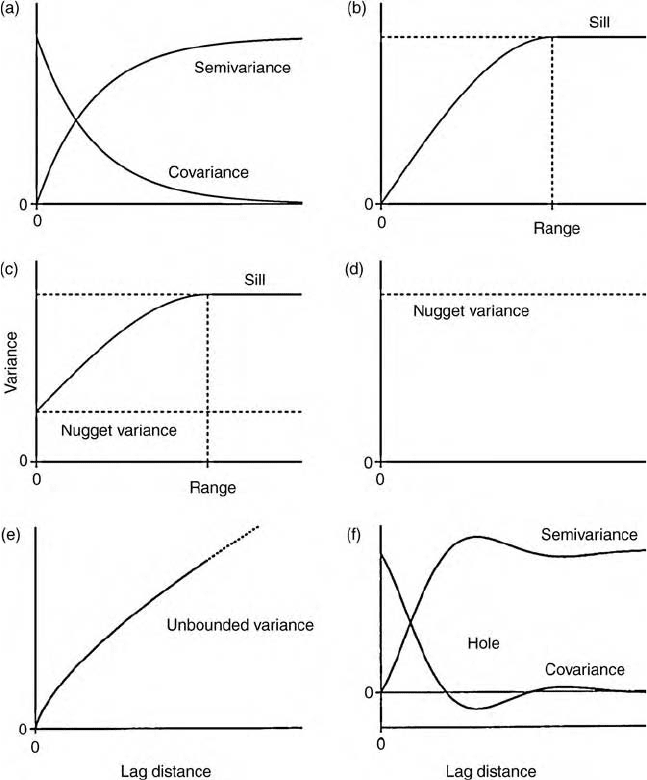
We now consider the more important characteristics of the covariance and

autocorrelation functions and the variogram. Figure 4.3 illustrates some of

these.

Autocorrelation. Like the ordinary product–moment correlation coefﬁcient, the

autocorrelation function varies between 1 and 1. From equation (4.9), its

value at lag 0 is 1.

Symmetry. Because of our assumption of stationarity,

CðhÞ¼E½fZðxÞmgfZðx þ hÞmg

¼ E½Zðx  hÞZðxÞm



¼ E½ZðxÞZðx  hÞm



¼ CðhÞ: ð4:17Þ

Characteristics of the Spatial Correlation Functions 55

In words, the autocovariance is symmetric in space. The same is true of the

variogram; i.e. gðhÞ¼gðhÞ for all h. So all three functions are even. This

means that we need consider only the positive lags, and indeed this is the

convention. In the graphs of the functions, such as those in Figure 4.3, we show

only the right-hand halves of the functions.

Figure 4.3 Theoretical functions for spatial correlation: (a) typical variogram and

equivalent covariance function; (b) bounded variogram showing the sill and range;

(e) unbounded variogram; (f) variogram and covariance function illustrating the hole

effect.

56 Characterizing Spatial Processes