Webster R., Oliver M.A., Geostatistics for Environmental Scientists

Подождите немного. Документ загружается.

land except where it is broken by water or rock. Measurements, in contrast, are

made on small cores or on bulked samples from small plots or ﬁelds. Similarly,

rainfall is recorded in small gauges separated from one another by large

distances. Data in this sense are fragmentary; they constitute a sample from

whatever region is of interest, and from them we can try to describe the region

in terms of mean values and variation.

The principal advances in sampling theory, sometimes known as classical

theory, were made in the 1930s. The aim was to estimate means, and to a lesser

extent higher-order moments, especially variances. It was not concerned to

express spatial variation, which has become the province of geostatistics.

Nevertheless, many of the ideas and form ulae for geostatistics derive from the

classical theory, and we therefo re devote a short section to them. For fuller

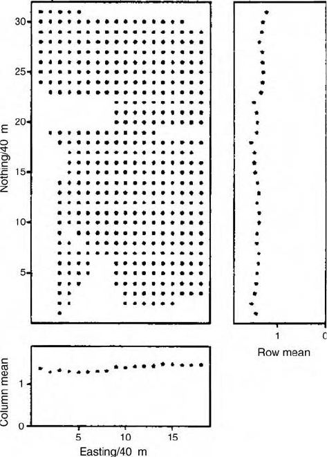
Figure 2.7 Posting of data for Broom’s Barn Farm with the row and column means

plotted on the right-hand side and at the bottom, respectively.

Sampling and Estimation 27

treatment you should consult one of the standard texts such as Cochran (1977)

and Yates (1981).

Better still in the context of environmental survey is the new book by de

Gruijter et al. (2006) which deals with spatial sampling for both design-

based estimation (the classical situation) and model-based prediction of

geostatistics.

2.6.1 Target population and units

Theﬁrststepinsamplingtheoryistodeﬁneatarget population. This population

comprises a set of units. In environmental survey a population is almost

always circumscribed by the boundary of a physical region, and the units are

all the places within it at which one might measure its properties. Measure-

ments must be made on bodies of material with ﬁnite size, and so there is a

ﬁnite numb er of non -o ver lap ping u ni ts in the p op ulat ion . The u nits ar e

usually so small in relatio n to the whole region that the popul a tion is

effectively inﬁnite. Millions of rain gauges 30 cm across could ﬁt into a region

of several hundred square kilometres without overlapping. The same is true of

boreholes and soil proﬁle pits. Even if the units were ﬁelds, there would be

thousands of them. Nevertheless, they are all large enough to encompass

variation, and in any on e survey they should be of the same size. In fact, they

should all hav e the s ame size, shape and ori enta t ion, known as th e support of

the sample.

The population is sam pled by taking a subset of its units on a deﬁned support.

In classical theory this subset must be chosen with some element of randomiza-

tion to ensure that the estimates from it are unbiased and to provide a

probabilistic basis for inference. Perhaps paradoxically, the units must be

selected according to a design to achieve this, and the technique is often called

‘design-based estimation’ in consequence.

2.6.2 Simple random sampling

This is the simplest form of design. Every unit in the sample is chosen without

regard to any other, and all units have the same chance of selection.

Estimates from a simple random sample

If there are N units in the sample then its mean,



z, estimates the mean of the

parent population, m,by

m ¼



z ¼

i¼1

: ð2:20Þ

28 Basic Statistics

The variance of the population is the expected mean squared difference between

m and z, i.e. it is the mean of ðz  mÞ

, denoted by s

. It is estimated by

¼ s

N  1

i¼1

ðz



zÞ

: ð2:21Þ

The divisor is N  1, not N, and this difference between the formula for the

estimated variance of a population and the variance of a ﬁnite set, equation (2.3),

arises because we do not know the true mean, but have only an estimate of it

from the data. The standard deviation of the sample, s, computed using equation

(2.21), estimates s. In like manner we estimate the population covariance

between two variables by replacing the divisor N in equation (2.10) by N  1.

Estimation variance and standard error

All estimates are subject to error: sample information is never complete, and we

want a measure of the uncertainty. This is usually expressed by the estimation

variance of a mean:



zÞ¼



zÞ¼s

=N: ð2:22Þ

It estimates the variance we should expect if we were to sample repeatedly and

compute the average squared difference between the mean m and the sample

mean,



E½s



zÞ ¼ E½ð



z  mÞ



¼ s

=N: ð2:23Þ

Its square root is the standard error, sð



zÞ. The equation introduces the symbol E

to signify the expected value of something.

Naturally, s



zÞ should be as small as possible. Evidently we can decrease



zÞ, and improve our estimates, by increasing N, the size of the sample. Unless

we can measure every unit in a population, however, we cannot eliminate the

error. Further, simply increasing N confers less and less beneﬁt for the effort

involved, and beyo nd about 25 the gain in precision is disappointing.

2.6.3 Conﬁdence limits

Having obtained an estimate and its variance we may wish to know within

what interval it lies for any degree of conﬁdence. If the variable has a normal

distribution and the sample is reasonably large then the conﬁdence limits for

the mea n are readily obtained as follows.

Sampling and Estimation 29

We consider a standard normal deviate, i.e. a normally distributed variable, y,

with a mean of 0 and variance of 1, sometimes written Nð0; 1Þ . Then for any m

and s,

y ¼

z  m

: ð2:24Þ

Conﬁdence limits on a mean are given by



z  ys=

ﬃﬃﬃﬃ

and



z þ ys=

ﬃﬃﬃﬃ

: ð2:25Þ

These are the lower and upper limits on m, given a sample mean



z and standard

deviation s that estimates s

precisely, corresponding to some chosen prob-

ability or level of conﬁdence. Values of standard normal deviates and their

cumulative probabilities are published, and we list the values for a few typical

conﬁdences at which people might wish to work and the associated values of y

in Table 2.3. The ﬁrst entry is usually too liberal, and we include it only to show

that approximately 68% of a normally distributed population lies within the

range s to þs.

2.6.4 Student’s t

With small samples s

is a poor estimate of s

, and in these circumstances

one should replace y in expressions (2.25) by Student’s t, which is deﬁned

t ¼



z  m

ﬃﬃﬃﬃ

: ð2:26Þ

The true mean, m, is unknown of course, but t has been worked out and

tabulated for N up to 120. So one chooses the conﬁdence level, and then ﬁnds

from the published table the value of t corresponding to N  1 degrees of freedom.

The conﬁdence limits of the mean are then



z  ts=

ﬃﬃﬃﬃ

and



z þ ts=

ﬃﬃﬃﬃ

: ð2:27Þ

As N increas es so t approaches y, and for N  60 the differences are trivially

small. So we need use t only when N < 60.

Table 2.3 Typical conﬁdences and their associated standard normal deviates, y.

Conﬁdence (%) 68 75 80 90 95 99

y 1.0 1.15 1.28 1.64 1.96 2.58

30 Basic Statistics

2.6.5 The x

distribution

Let y

; y

; ...; y

be m values drawn from a standard normal distribution. Their

sum of squares is

i¼1

: ð2:28Þ

This quantity has the distribution

f ðxÞ¼f2

f =2

G ðf =2Þg

1

ðf =2Þ1

expðx=2Þ for x  0; ð2:29Þ

where f is the number of degrees of freedom, equal to N  1 in our case, and G

is the gamma function deﬁned for any k > 0by

G ðkÞ¼

k1

expðxÞdx:

Values of x

have been worked out and tabulated, and can be found in any

good book of statistical tables, such as that by Fisher and Yates (1963). They

are also available in many statistical packages on computers.

The variance estimated from a sample is, from equation (2.21),

N  1

i¼1

ðz

 m Þ

: ð2:30Þ

Dividing through by s

gives

N 1

i¼1

ðz

 m Þ

; ð2:31Þ

and so

¼ x

=ðN  1Þ and x

¼ðN 1Þs

with N  1 degrees of freedom, provided the original population was normally

distributed.

Rearranging the last expression gives the following limits for a variance:

ðN  1Þs

 s



ðN  1Þs

; ð2:32Þ

Sampling and Estimation 31

where p

and p

are the probabilities and for which we can obtain values of x

from the published tables.

2.6.6 Central limit theorem

In the foregoing discussion of conﬁdence limits (Section 2.6.3) we have

restricted the formulae to those for the normal distribution, the properties of

which are so well established. It lends we ight to our argument for transforming

variables to normal if that is possible. However, even if a variable is not

normally distributed it is often still possible to use the tabulated values and

formulae when working with grouped data. As it happens, the distributions of

sample means tend to be more nearly normal than those of the original

populations. Further, the bigger is a sample the closer is the distribution

of the sample mean to normality. This is the central limit theorem. It

means that we c an use a l arge body of t he ory w he n stud ying s am ple s from

the r eal world.

We might, of course, have to work with raw data that cannot readily be

transformed to normal, and in these circumstances we should see whether the

data follow some other known distribution. If they do then the same line of

reasoning can be used to arrive at conﬁdence limits for the parameters.

2.6.7 Increasing precision and efﬁciency

The conﬁdence limits on means computed from simple random samples can be

alarmingly wide, and the sizes of sample needed to obtain satisfactory precision

can also be alarmingly large. One reason when sampling space with a simple

random design is that it is inefﬁcient. Its cover is uneven; there are usually parts

of the region that are sparsely sampled while elsewhere there are clusters of

sampling points. If a variable z is spatially auto correlated, which is likely at some

scale, then clustered points duplicate information. Large gaps between sampling

points mean that information that could have been obtained is lacking.

Consequently, more poin ts are needed to achieve a given precision, as measured

by s



zÞ, than if the points are spread more evenly. There are several better

designs for areas, and we consider the two most common one s, stratiﬁed random

and systematic.

Stratiﬁed sampling

In stratiﬁed designs the region of interest, R, is divided into small subdivisions

(strata). These are typically small squares, but they may be other shapes, of

equal area. At least two sampling points are chosen ran domly within each

stratum. For this scheme the largest possible gap is then less than four strata.

32 Basic Statistics

The variance within a stratum k is estimated from n

data in it by

 1

i¼1

ðz



; ð2:33Þ

in which z

are the measured values and



is their mean. If there are K strata

then by averaging their variances we can obtain the estimated variance for the

region:



z; stratifiedÞ¼

k¼1

: ð2:34Þ

Its square root is the standard error.

The quantity ð1=KÞ

k¼1

is the pooled within-stratum variance, denoted

by s

. If there is any spatial dependence then it will be less than s

, and so the

variance and standard error of a stratiﬁed sample will be less than that of a

simple random sample for the same effort, the same size of sample.

The ratio s



zÞ=s



z, stratiﬁed) is the relative precision of stratiﬁcation.

If we were happy with the precision achieved by simple random sampling

then we could get the same precision by stratiﬁcation with a smaller sample.

Stratiﬁed sampling is more efﬁcient by the factor

random

stratified

Systematic sampling

Systematic sampling provides the most even cover. In one dimension the

sampling points are placed at equal intervals along a line, a transect. In two

dimensions the points may be placed at the intersections of an equilateral

triangular grid for maximum precision or efﬁciency. With this conﬁguration the

maximum distance between any unsampled point and the nearest poin t on the

sampling grid is the least. However, rectangular grids are more practical, and

the loss of precision compared with triangular ones is usually so small that they

are preferred.

The main disadvantage of systematic sampling is that classical theory

provides no means of determining the variance or standard error without

bias from the sample because once one sampling point has been chosen (and

the orientation in two dimensions) there is no randomization. An approxima-

tion may be obtained by dividing the region into strata and computing the

pooled within-stratum variance as if sampling were random within the strata.

The result will almost certainly be an overestimate, and conservative therefore.

A closer approximation, and one that will almost certainly be close enough, can

usually be obtained by Yates’s method of balanced differences (Yates, 1981).

Sampling and Estimation 33

Estimates of error by balanced differences are computed as follows. Consider

ﬁrst regular sampling on a transect, i.e. in one dimension. The transect is

viewed through a small window containing, say, m sampling points with values

; z

; ...; z

. We then compute for the window the differences:

 z

þ z

 z

þþ

: ð2:35Þ

A value of m ¼ 9 is convenient. We then move the window along the transect

in steps and compute d

at each new position. If the transect is short then the

positions should overlap; if not, a satisfactory procedure is to choose the ﬁrst

sampling point in a new position as the last one in the previous position. In this

way every sampling point contributes, and with equation (2.35) all contribute

equally. Then the variance for the transect mean is the sum

ðbalanced differencesÞ¼

Jðm  2 þ 0:5Þ

J¼1

; ð2:36Þ

where J is the number of steps or positions of the window, and the quantity

m  2 þ 0:5 is the sum of the squares of the coefﬁcients in equation (2.35).

For a two-dimensional grid the procedure is analogous. One chooses a square

window. For illustration let it be of side 4. The coefﬁcients can be assigned as

follows:

0:25 þ0:5 0:5 þ0:25

þ0:5 1:0 þ1:0 0:5

0:5 þ1:0 1:0 þ0:5

þ0:25 0:5 þ0:5 0:25

The variance is calculated as in equation (2.36), now with the divisor J 6:25,

the value 6.25 being the sum of the squares of the coefﬁcients above. Again, the

positions of the window may overlap, but usually it is sufﬁcient to arrange them

so that only the sides are in common, and with this arrangement and the

coefﬁcients listed all points count and carr y equal weight.

What these schemes do in both one and two dimensions, and in three if the

scheme is extended, is to ﬁlter out long-range ﬂuctuation, just as stratiﬁcation

does.

Where there is trend across the sampled region or periodicity, as, for example,

in an orchard or as a result of land drainage, systematic sampling can give

biased estimates of means. Such bias can be avoided by randomizing system-

atically within the grid. The result is unaligned sampling (see Webster and Oliver,

1990). It gives almost even cover. The disadvantage is the same as that of strict

grid sampling in that the error cannot be estimated very accurately. The best

procedure again is to stratify the region and compute the pooled within-stratum

34 Basic Statistics

variance. Empirical studies have shown some big gains in precision and

efﬁciency from both systematic and unaligned sampling (again, see Webster

and Oliver, 1990, for an example).

2.6.8 Soil classiﬁcation

Another way of stratifying a region to improve the precision of estimates is to

divide it on the basis of certain attributes. This practice is widespread in land

resource surveys, and it was the norm in soil survey. Soil surveyors stratify, i.e.

classify, regions on the appearance of the soil in proﬁle and on related features

in the landscape.

Regional mean

If the classiﬁcation is good then the within-class variance of a stratum, i.e. the

pooled within-stratum variance, is smaller than the total variance. Classiﬁca-

tion should therefore improve the precision or efﬁciency in estimating the

regional mean.

The classes of soil are rarely equal in area, and so the formula, equation

(2.34), must be adjusted accordingly. We deﬁne a weight, w

, for the kth

stratum or class in proportion to the area it covers:

area of stratum k

total area

The mea n, m, for the whole area is then estimated by the weighted average:



z ¼

k¼1



; ð2:37Þ

where



is the estimated mean of the kth stratum. The estimation variance is



z; stratifiedÞ¼

k¼1

()

: ð2:38Þ

The average within-class varianc e and other diagnostics of a classiﬁcation can

be estimated from data by analysis of variance, which is both elegant and

powerful. It can also serve for prediction, and we therefore defer its treatment to

the next chapter.

Sampling and Estimation 35