Webster R., Oliver M.A., Geostatistics for Environmental Scientists

Подождите немного. Документ загружается.

Positive semideﬁniteness. The covariance matrix for any number of points is

positive semideﬁnite. That is to say that for a matrix of order n its determinan t

Cðx

; x

Þ Cðx

; x

Þ  Cðx

; x

Cðx

; x

Þ Cðx

; x

Þ  Cðx

; x



Cðx

; x

Þ Cðx

; x

Þ  Cðx

; x



and all its principal minors are positive or zero. This is necessary because the

variance of any linear sum of the random variables,

YðxÞ¼l

Zðx

Þþl

Zðx

Þþþl

Zðx

Þ; ð4:18Þ

must be positive or zero; a variance cannot be negative. The covariance and

autocorrelation functions are positive semideﬁnite. In like manner, the vario-

gram must be negative semideﬁnite. We shall develop this in Chapter 5 where

we shall see that this limits the choice of legitimate mathematical functions to

describe the covariance function.

Continuity. As mentioned above, most environmental variables are continu-

ous; the stochastic processes that we believe to represent them are continuous,

and so also are the autocovariance functions and variograms of a continuous

lag. Crucially, CðhÞ and gðhÞ are continuous at h ¼ 0, and if that is so they

must be continuous everywhere. So CðhÞ decline s from some positive value,

Cð0Þ¼s

,at0 to smaller values at lon ger lag distances; see Figure 4.3(a). Its

mirror image, the variogram, increases from 0 at h ¼ 0, i.e. it must pass

through the origin if the process is continuous; see Figure 4.3(a)–(b).

If this were not so then we should have a continuous sequence of positions in

space, the values at which are not related. It seems impossible, yet in practice

data often suggest that a spatial process is discontinuous. It manifests itself most

evidently in the sample variogram; the calculated values appear to approach

some positive value on the ordinate as the lag distance approaches 0, whereas,

at h ¼ 0, gð0Þ must be 0; Figure 4.3(c). This discrepancy is known as the

nugget variance. The term arose in gold mining from the notion that gold

nuggets occur qui te independently of one another at random; they are sparse

and certainly not continuous at the working scale. They have a variance that

jumps from 0 at lag zero to positive immediately away from the origin, and we

can reco gnize this by deﬁning

gðhÞ¼s

f1  dðhÞg; ð4:19Þ

where dðhÞ is the Kronecker delta function taking the values 1 when h ¼ 0 and

0 otherwise.

Characteristics of the Spatial Correlation Functions 57

The data themselves differ from their neighbours in irregular steps, large or

small, rather than in smooth progression. It seems as though they derive from

two or more components, one uncorrelated superimposed on another that is

correlated. In other words, we seem to have one source of variation in which

contiguous positions in space do take values of Z that are totally unrela ted.

Engineers recognize this uncorrelated variation as ‘white noise’. They usually

express it by its covariance function:

CðhÞ¼s

dðhÞ; ð4:20Þ

where now dðhÞ is the Dirac function taking the values 0 when jhj 6¼ 0 and

inﬁnity when jhj¼0. Thus for white noise CðhÞ¼0 for all jhj > 0 and

Cð0Þ¼1. The representation might seem bizarre, but it is the only way that

we can describe white noise using covariances. Its equivalent is a ‘pure nugget’

variogram; Figure 4.3(d).

For properties that vary continuously in space, such as the soil’s pH, the

concentrations of trace metals, air temperature and rainfall, the apparent nugget

variance comprises measurement error plus variation that occurs over distances

less than the shortest sampling interval. The latter is usually dominant.

Monotonic increasing. The variograms in Figure 4.3(b)–(c) are monotonically

increasing functions, i.e. the variance increases with increasing lag distance.

The small values of gðhÞ at short jhj show that the ZðxÞ are similar, and that as

jhj increases ZðxÞ and Zðx þ hÞ become increasingly dissimilar on average.

Looked at from the point of view of correlation, rðhÞ increases as the lag

distance sho rtens, and the process is therefore said to be autocorrelated or

spatially dependent.

Sill and range . The variograms of second-order stationary processes reach

upper bounds at which they remain after their initial increases, as in Figure

4.3(b)–(c). The maximum is known as the sill variance; it is the a priori

variance, s

, of the process.

A variogram may reach its sill at a ﬁnite lag distance, in which case it has a

range, also known as the correlation range since this is the range at which the

autocorrelation becomes 0; Figure 4.3(c). This separation marks the limit of

spatial dependence. Places further apart than this are spatially independent.

Some variograms approach their sills asymptotically, and so they have no strict

ranges. For practical purposes their effective ranges are usually taken as the lag

distances at which they reach 0.95 of their sills.

Unbounded variogram. If, as in Figure 4.3(e), the variogram increases indeﬁ-

nitely with increasing lag distance then the process is not second-order

stationary. It might be intrinsic, but the covariance does not exist.

Hole effect. In some instances the variogram decreases from its maximum to a

local minimum and then increases again, as in Figure 4.3(f). This maximum is

58 Characterizing Spatial Processes

equivalent to a minimum in the covariance function, which appears as a ‘hole’.

This form arises from fairly regular repetition in the process. A variogram that

continues to ﬂuctuate with a wave-like form with increasing lag distance

signiﬁes greater regularity.

Anisotropy. Spatial variation is not necessarily the same in all directions. If the

process is anisotropic then so is the variogram, as is the covariance function if it

exists. Anisotropy may take several forms. The initial gradient may vary. If the

variogram has a sill then variation in the gradient will lead to variation in the

range, or effective range. If the variation with changing direction is such that a

simple transformation of the spatial coordinates will remove it then we have

geometric anisotropy (see Chapter 5).

A region may contain preferentially oriented zones with different mean

values. In these circumstances the variance enc ountered changes with change

in direction so that the sill ﬂuctuates. This is called zonal anisotropy.

Trend. In some instances the experimental variograms (see below for their

deﬁnition) follow smooth curves that approach the origin with decreasing

gradient: the curves have concave upwards forms. This shape can arise from

local trend or drift, i.e. smooth change in the underlying variable. The dashed line

in Figure 5.3 is an example. In other instances the experimental estimates

increase sharply after having appeared to reach sills, as in Figure 9.2(a); this

is often a sign of long-range trend in the variation superimposed on

relatively short-range random variation. In both circumstances the expected

value, E½ZðxÞ, is not constant, even within small neighbourhoods, but is a

function of position. We have then to elaborate our model for spatial variation to

ZðxÞ¼uðxÞþ" ðxÞ: ð4:21Þ

The quantity uðxÞ is the local trend, and it replaces the means in equatio ns

(4.10) and (4.16). The assumption of second-order stationarity does not hold,

nor does the intrinsic hypothesis. The experimental semivar iances calculated

from the raw data no longer estimate the expected squ ared differences between

the resi duals at two places. The residuals are given by

"ðxÞ¼ZðxÞuðxÞ: ð4:22Þ

They constitute the random process with its associat ed variogram,

gðhÞ¼

E f"ðxÞ"ðx þ hÞg

: ð4:23Þ

A more general description of non-stationarity is as an intrinsic random

function of order k (IRFk):

ZðxÞ¼Z

ðxÞþuðxÞ: ð4:24Þ

Characteristics of the Spatial Correlation Functions 59

We describe some ways of dealing with the difﬁculties of non-stationarity in

Chapter 9.

4.7 WHICH VARIOGRAM?

The variogram (and covariance function) as treated above is a function of an

underlying stochastic process. We may regard it as the theoretical variogram.It

may be thought of as the average of the variograms from all poss ible realiza-

tions of the process. Following Matheron (1965), we need to distinguish it from

two others, namely the regional and the experimental.

The regional variogram is the variogram of the particular realization in a ﬁnite

region, R. It is the one that you might compute if you had complete information

of the region, as, for example, from the simulated ﬁelds in Figures 5.5, 5.6, 5.8

and 5.11, and from many digital ima ges (see Mun˜ oz-Pardo, 1987). The

regional variogram does not necessarily represent the whole ensemble. A

process that is second-order stationary might appear unbounded in a small

region, especially if the distance across the region is smaller than the correlation

range. The regional variogram is called the non-ergodic variogram by some

workers, e.g. Brus and de Gruijter (1994), for this reason. It is more or less

accessible, depending on the effort we are prep ared to devote to sampling the

realization, and this leads us to the third variogram, below.

The experimental variogram is computed from data, zðx

Þ; i ¼ 1; 2; ... , which

constitute a sample from the region. It is also called the sample variogram.We

describe it in Section 4.9. It necessarily applies to an actual realization, and it

estimates the regional variogram for that realization. It is usually the only

variogram that we know, and any inference from it requires modelling, as

described in Chapter 5.

4.8 SUPPORT AND KRIGE’S RELATION

Spatial dependence within a ﬁnite region has both theoretical and practical

consequences, which we now explore.

The variance of ZðxÞ within a region R of area jRj is the double integral of the

variogram:



gðR; RÞ¼

jRj

gðx  x

Þdxdx

; ð4:25Þ

where x and x

sweep independently over R. In geostatistics this variance is

called the dispersion variance of ZðxÞ in R. Unless the variogram is all nugget the

dispersion variance for a ﬁnite R is less than the a priori variance of the process,

60 Characterizing Spatial Processes

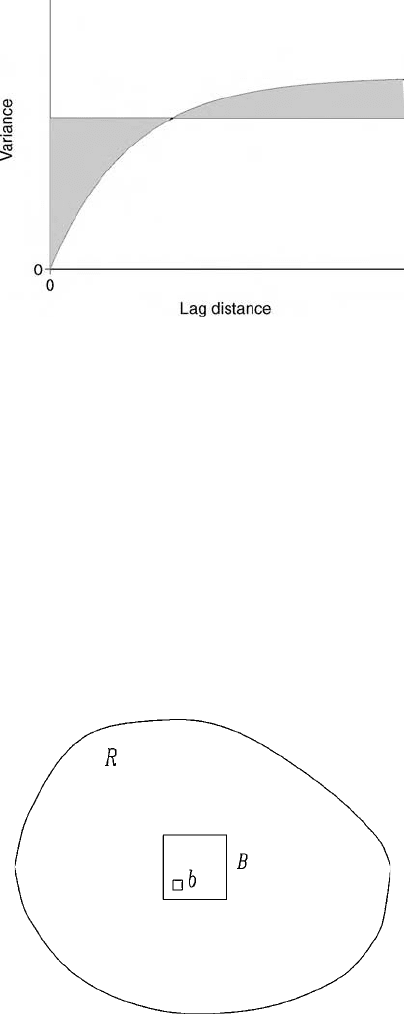
if it is second-order stationarity. Figure 4.4 shows the relation between the two

for a one-dimensional process; in it the shaded areas are equal. Evidently, as R is

made smaller s

diminishes, until in the limit we are left with a point, at which

disappears.

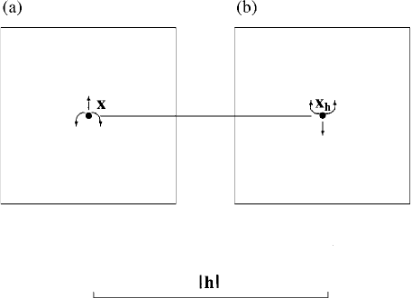
The region R (see Figure 4.5) limits the extent of a realization . At the small

end of our spatial scale we encounter another limit. Measurements must be

made on ﬁnite volumes, whether of samples taken into the laboratory or the

surroundings of instruments placed in the ﬁeld. The volume, with its particular

size, shape and orientation, is known as the support of the sample. The supports

have ﬁnite cross-sectional areas in R

, and they are effectively small but ﬁni te

regions, each with its own dispersion variance. If we denote them by b, each

Figure 4.4 Relation between the variogram and the dispersion variance in a ﬁnite

region, R.

Figure 4.5 Krige’s relation for a region, R, a block, B, and a small support, b.

Support and Krige’s Relation 61

with area jbj (see Figure 4.5), then their dispersion variances are given by the

analogue of equation (4.25):



gðb; bÞ¼

jbj

gðx  x

Þdxdx

: ð4:26Þ

One practical consequence of this is that the support of the sample sets a

minimum to the resolution of the spatial variation that can be detected and

measured by that sample: engineers will understand this as ‘band-limited’

measurement.

In many ap plic ations we are interested in b lock s, B, of intermediate size, jBj

(see Figure 4.5). They may be mini ng blocks, plots in an experiment, or ﬁelds

on a farm, as example s. They too will have dispersion variance s, s

,deﬁnedin

a way analogous to s

and s

, and with inter medi ate values. W e n ow relate

the th ree.

Consider ﬁrst the supports b. Though small, they have ﬁnite size, and so in a

ﬁnite region they are ﬁnite in number if they do not overlap. If there are n

them with values z

; i ¼ 1; 2; ...; n

; then their variance in R is

ðb 2 RÞ¼

i¼1



 z

; ð4:27Þ

where



is the mean of the z

. In like manner their variance in a block B with

mean



ðb 2 BÞ¼

i¼1



 z

; ð4:28Þ

which can be averaged over all B 2 R to give



ðb 2 BÞ. Finally, we consider the

blocks, B, themselves. Their variance in R is

ðB 2 RÞ¼

j¼1







; ð4:29Þ

where



is the mean of Z in the jth block.

For any ﬁnite region that is divided in the above way into blocks, which in

turn are further subdivided, whether into small supports or sma ller blocks, the

dispersion variance is partitioned quite simply as

ðb 2 RÞ¼



ðb 2 BÞþs

ðB 2 RÞ: ð4:30Þ

In words, the dispersion variance of Z of supports b in region R is the sum of the

variance of the supports with blocks B plus the variance of the blocks within R.

This is Krige’s relation. It is strictly analogous to the partition of the total

62 Characterizing Spatial Processes

variance into within and between classes in the simple one-way analysi s of

variance.

The expectations of the dispersion variances are all read ily obtained from the

variogram by

ðb 2 RÞ¼



gðR; RÞ



gðb; bÞ;

ðB 2 RÞ¼



gðR; RÞ



gðB; BÞ;

ðb 2 BÞ¼



gðB; BÞ



gðb; bÞ;

ð4:31Þ

and so Krige’s relation applies to them equally.

4.8.1 Regularization

Another consequence of the ﬁnite sample support is that the variogram in

practice is a function of the support. The larger the support is the more

variation each measurement encompasses, and the less there is in the inter-

vening space to appear in the variogram. This inevitably diminishes the sill or

gradient and tends to make the variogram concave upwards near to the origin.

It is a physical regularization, the statistical aspects of which we describe below.

Results should always refer speciﬁcally to the particular support, which should

therefore remain the same throughout any one investigation.

The variogram on one support can be related, at least theoretically, to that on

another. The semivariance for two supports bðxÞ and bðx þ hÞ, the centroids of

which are h apart, is

ðhÞ¼E½fZ

ðxÞZ

ðx þ hÞg

; ð4:32Þ

where Z

ðxÞ and Z

ðx þhÞ are the integrals of ZðxÞ over the supports b. This is

composed of two parts, the average squ ared difference between the points in

one support and those in the other less the dispersion variance within supports.

The ﬁrst is given by



gðb; b

Þ¼

jbj

gðx  x

Þdxdx

; ð4:33Þ

where x sweeps one support and x

sweeps the other indepen dently, as

in Figure 4.6. The second is the integral of the variogram within the support



gðb; bÞ¼

jbj

gðx  x

Þdxdx

; ð4:34Þ

Support and Krige’s Relation 63

where x and x

sweep b independently, illustrated in Chapter 8 (Figure 8.1). The

variogram on the new supports thus becomes

ðhÞ¼



gðb; b

Þ



gðb; bÞ: ð4:35Þ

If jhj is large relative to the distances across the support then



gðb; b

Þ is

approximately the punctual semivariance at lag h, and

ðhÞgðhÞ



gðb; bÞ: ð4:36Þ

So when jhj

ﬃﬃﬃﬃﬃﬃﬃﬃﬃﬃﬃﬃﬃﬃﬃﬃﬃﬃ

area of b

the regularized variogram is derived from the

punctual one sim ply by s ubtrac tion of the dispersion varia nce of the

support.

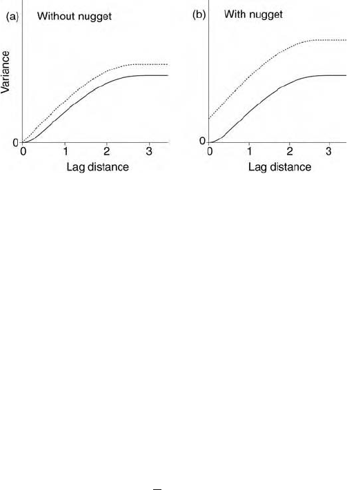
This procedure in which the variogram for one support is obtained from that

of a smaller support is known as regu larization. Figure 4.7 shows what can

happen to the variogram. In this ﬁgure two punctual variograms appear as the

dashed lines, (a) without a nugget component and (b) with one. The solid lines

are variograms derived by regularization with blocks of size 0:5  0:5 units.

Notice the sills are diminished, the nugget variance disappears and the

approach of the variogram at the origin is somewhat concave upwards. It is

especially important when bulking samples, for two reasons. The ﬁrst is that the

supports can be large. Second, if the variogram is known for very small supports

on which the variable has been measured then that for samples bulked over

larger areas, the regularized variogram, can be determined from it and surveys

be planned with greater efﬁciency.

Figure 4.6 The block-to-block integration of the variogram.

64 Characterizing Spatial Processes

4.9 ESTIMATING SEMIVARIANCES AND COVARIANCES

As mentioned above, the variogram is the cornerstone of geostatistics, and it is

therefore vital to estimate, interpret and model it correctly. This section

concerns its estimation using the usual computing equation, Matheron’s

method-of-moments estimator, and how it applies to various kinds of sampling.

We also describe how to determine the possible presence of anisotropy and non-

stationarity in the process of interest.

4.9.1 The variogram cloud

For any set of data we can compute the variances for every pair of points, x

and

,as

gðx

; x

Þ¼

fzðx

Þzðx

Þg

: ð4:37Þ

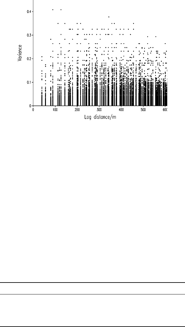
These values can then be plotted against the lag distance as a scatter diagram,

called the ‘variogram cloud’ by Chauvet (1982). Figure 4.8 shows the variogram

cloud for log

K at Broom’s Barn to a lag of 600 m. It contains all of the

information on the spatial relations in the data to that lag. In principle we could

ﬁt a model to it to represent the regional variogram, but in practice it is almost

impossible to judge from it if there is any spatial correlation present, what form it

might have, and how we could model it. A more practicable approach is to

average the variances for each of a few lags and then examine the result.

Nevertheless, the variogram cloud shows the spread of values at each lag, and it

might enable us to detect outliers or anomalies. The tighter this distribution is the

stronger is the spatial continuity in the data.

Figure 4.7 Regularization of punctual variograms (dashed) to ones with block supports

of 0:5  0:5 (solid lines): (a) without a nugget component; (b) with a nugget component.

Estimating Semivariances and Covariances 65

4.9.2 h-Scattergrams

The h-scattergram of zðxÞ plotted against zðx þ hÞ for each lag interval shows

the joint distribution of pairs of points that interval apart as mentioned above

(section 4.3.1), which represents the pdf. The closer the points lie to the

diagonal line with gradient 1, the stronger is the correlation,

rðhÞ, and the

smaller is the semivariance,

gðhÞ. Figure 4.9 shows the h-scattergrams for four

lag intervals, 40 m, 80 m, 120 m and 160 m, computed from the data on

log

K on Broom’s Barn Farm. The autocorrelation coefﬁcients and semivar-

iances listed in Table 4.1 describe quantitatively what happens as the lag

interval increases; the correlations between pair s of points decrease and the

semivariances increase.

Figure 4.8 The variogram cloud of log

K at Broom’s Barn Farm.

Table 4.1 Autocorrelation coefﬁcients and semivariances for log

Kat

Broom’s Barn Farm computed for lag distances 40 m (lag 1), 80 m (lag 2),

120 m (lag 3) and 1600 m (lag 4).

Lag distance/m Autocorrelation coefﬁcient Semivariance

40 0.590 0.00726

80 0.470 0.00942

120 0.399 0.01065

160 0.311 0.01228

66 Characterizing Spatial Processes