Webster R., Oliver M.A., Geostatistics for Environmental Scientists

Подождите немного. Документ загружается.

Modelling the Variogram

In Chapter 4 we saw that when we compute an empirical variogram we obtain

an ordered set of values, the experimental or sample variogram, consisting of

gðh

Þ;

gðh

Þ; ...; at particular lags, h

; h

; .... This variogram summarizes the

spatial relations in the data. We usually want more than that, however; we

want a vari ogram to describe the variance of the region. Each calculated

semivariance for a particular lag is only an estimate of a mean semivariance for

that lag. As such it is subject to error.

This error, which arises largely from sampling ﬂuctuation, can give the

experimental variogram a more or less erratic appearance, as depicted by the

plotted points in the graphs in the left-hand column of Figure 5.1. We computed

this experimental variogram from 87 values of log

K from the Broom’s Barn

data by taking every ﬁfth value from the ﬁle. In the right-hand column is the

experimental variogram computed from all 434 data; the points lie on a

relatively smooth curve. Evidently the sampling ﬂuctuation is more pronounced

where the data points are further apart and there are fewer of them. We explore

the effects of the number of data points on the reliability of the variogram in

more detail in Chapter 6, and we explain the smooth curves drawn through the

experimental values later in this chapter.

The true variogram representing the regional variation is continuous, and it

is this vari ogram that we should really like to know. We can use our observed

values as approximations to the function by imagining a curve passing through

them, such as the ones we have drawn in Figure 5.1. In two dimensions we

have to imagine a surface, for the variogram of a two-dimens ional ﬁeld is itself

two-dimensional. How closely should we attempt to follow the experimental

variogram? Answering this is difﬁcult because we do not know how much of

the obse rved ﬂuctuation is due to error and how much is structural.

The solution usually taken is that of Occam’s razor; namely, ﬁt the simplest

function that makes sense, subject to certain mathematical constraints which

are considered below. We ignore the point-to-point ﬂuctuation and concentrate

on the general trends.

Geostatistics for Environmental Scientists/2nd Edition R. Webster and M.A. Oliver

# 2007 John Wiley & Sons, Ltd

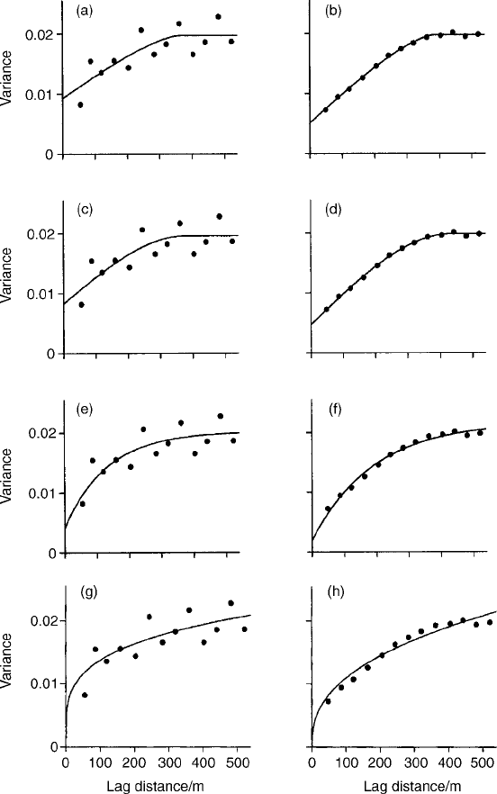
Figure 5.1 Experimental variograms plotted, as points, of log

K at Broom’s Barn

computed from 87 data in the left-hand column and from all 434 data in the right-hand

column. The solid lines from top to bottom are: the circular, spherical, exponential and

power models ﬁtted to them.

78 Modelling the Variogram

Another reason for ﬁtting a continuous function is to describe the spatial

variation so that we can estimate or predict values at unsampled places and in

larger blocks of land optimally by kriging (see Chapter 8). This requires

semivariances at lags for which we have no direct comparisons, and we must

be able to calculate these from such a function. The function must therefore be

mathematically deﬁned for all real h.

There are a few principal features that a function must be able to represent.

These include:

(1) a monotonic increase with increasing lag distance from the ordinate of

appropriate shape;

(2) a constant maximum or asymptote, or ‘sill’;

(3) a positive intercept on the ordinate, or ‘nugget’;

(4) periodic ﬂuctua tion, or a ‘ho le’;

(5) anisotropy.

5.1 LIMITATIONS ON VARIOGRAM FUNCTIONS

5.1.1 Mathematical constraints

Not any close-ﬁtting function will serve. The model we choose must describe

random variation, and the function must be such that it will not give rise to

‘negative variances’ of combinations of random variables. This is explained

below.

Let zðx

Þ; i ¼ 1; 2; ...; n; be a realization of the random variable ZðxÞ

with covariance function CðhÞ and variogram gðh Þ. Now consider the linear

sum

y ¼

i¼1

zðx

Þ;

where the l

are any arbitrary weights.

The vari able Y from which y derives is itself random with variance

var½Y¼

i¼1

j¼1

Cðx

 x

Þ; ð5:1Þ

where Cðx

 x

Þ is the covariance of Z betw een x

and x

. The variance of Y

may be positive or zero; but it may not be negative. The right-hand side of

equation (5.1) mu st ensure this. The covariance function, CðhÞ, must be positive

semideﬁnite. Equation (5.1) can be written

var½Y¼l

Cl  0; ð5:2Þ

Limitations on Variogram Functions 79

where l is the vector of weights and C is the matrix of covariances. If the latter is

positive semideﬁnite then so is the covariance function. In fact, since we are dealing

with ‘variables’, the variance cannot be zero, and so CðhÞ must be positive deﬁnite.

If the covariance does not exist, because the variable is intrinsic only and not

second-order stationary, then we rewrite equation (5.1) as

var½Y¼Cð0Þ

i¼1

j¼1



i¼1

j¼1

gðx

 x

Þ; ð5:3Þ

where gðx

 x

Þ is the semivariance of Z between x

and x

. The ﬁrst term on

the right-hand side of equation (5.3) contains Cð0Þ, the covariance at lag 0,

which we do not know, but we can eliminate it by making the weights sum to 0

without loss of generality. Then

var½Y¼

i¼1

j¼1

gðx

 x

Þ: ð5:4Þ

This may not be negative either; but notice the minus sign. So, the variogram

must be conditional negative semideﬁnite (CNSD), the condition being that the

weights in equation (5.4) sum to zero.

Only functions that ensure non-zero variances may be used for variograms. They

are called authorized models or functions in much of the literature.

5.1.2 Behaviour near the origin

The way in which the variogram approaches the origin is determined by the

continuity (or lack of continuity) of the variable, ZðxÞ, itself. We may

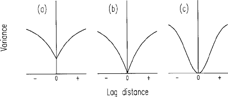
distinguish the following features, which are illustrated in Figure 5.2. As

mentioned in Chapter 4, the variogram is symmetric about the origin, and

for reasons that will become evident both halves appear in this ﬁgure.

Figure 5.2 Behaviour of the variogram near to the origin: (a) postive intercept

(nugget); (b) linear approach, not differentiable; (c) continuous and differentiable.

80 Modelling the Variogram

Positive intercept. The semivariance at jhj¼0 is by deﬁnition 0. It often happens,

however, that any line or surface projected through the experimental values to

the ordinate intersects it at some positive value, as in Figure 5.2(a). This implies a

discontinuity in ZðxÞ. The feature appeared often in gold mining, and the mining

engineers attributed it to the spatially independent occurrence of gold nuggets in

ore bodies. They called the phenomenon the ‘nugget effect’ and the intercept

‘nugget variance’. It is easy to imagine discontinuities arising from the dispersal of

small nuggets of gold in a large body of rock. The same might be true for

certain features of the soil, such as stones and concretions among the ﬁne earth.

Discontinuities in the soil’s physical and chemical properties are harder to

imagine, and any apparent nugget variance usually arises from errors of

measurement and spatial variation within the shortest sampling interval.

Linear approach. The variogram may approach the origin approximately linearly

with decreasing lag distance:

gðhÞbjhj as jhj!0; ð5:5Þ

where b is the gradient. The variogram passes through the origin, as in Figure

5.2(b), unlike in Figure 5.2(a), but its ﬁrst derivative is discontinuous there: its

gradient changes abruptly from negative to positive. Nevertheless, it signiﬁes

continuity in ZðxÞ itself, and because

lim E½fZðxÞZðx þ hÞg

¼0asjhj!0; ð5:6Þ

ZðxÞ is often said to be ‘mean-square’ continuous. It is not differentiable,

however, nor is the process it describes because it is random (see Chapter 4).

Parabolic approach. Figure 5.2(c) illustrates the situation in which a variogram is

parabolic at the origin; it passes smoothly through the origin with a gradient of

0 there, so that

gðhÞ¼bjhj

as jhj!0: ð5:7Þ

The variogram is twice differentiable at the origin, and ZðxÞ is itself differenti-

able: it varies smoothly, and it is no longer random. The exponent 2 represents

a strict limit to power functions for describing random processes.

A raw variogram that appears parabolic at the origin suggests that there is

local trend, i.e. short-range deterministic variation. This feature is described in

Chapter 4, and we deal with it again in Chapter 9. The expectation of ZðxÞ is

not stat ionary but depends on position x, thus:

E½ZðxÞ ¼ uðxÞ; ð5:8Þ

from equation (4.21).

Limitations on Variogram Functions 81

5.1.3 Behaviour towards inﬁnity

The way that a variogram behaves with increasing lag distance is constrained by

lim

gðhÞ

jhj

¼ 0asjhj!1: ð5:9Þ

The variogram must increase less than the square of the lag distance as the

latter approaches inﬁnity; if it does not then the process is not entirely random.

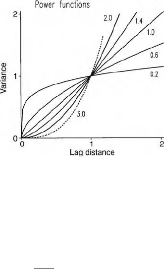
The limit is shown in Figure 5.3, in which the parameter a in the power

function is set to 2. Any function that increases more, such as that shown by

the dashed line with a ¼ 3, is not CNSD and so is not compatible with the

intrinsic hypothesis.

A variogram that increases faster than jhj

suggests that there is long-range

trend, again deterministic in the statistical sense (see Chapters 4 and 6). As

above, the expectation of ZðxÞ is not stationary but depends on position x; see

equation (5.8).

5.2 AUTHORIZED MODELS

There are two main families of simple functions that encompass the feat ures

listed above and that are CNSD. One represents unbounded variation, the other

bounded. We deal with them in turn in their isotropic form, so that the lag

vector jhj becomes a scalar measure in distance only, h. All of the ones that we

describe are used in practice.

Figure 5.3 Graphs of the power function, gðhÞ¼wh

, with a ¼ 0:2; 0:6; 1:0; 1:4;

and 2.0 (the limiting value for a), and with w set to 1, shown by solid lines. The dashed

line represents gðhÞ¼h

and is not an authorized function for a variogram.

82 Modelling the Variogram

5.2.1 Unbounded random variation

The idea of unbounded, i.e. inﬁnite, variance may seem strange. After all, we live

on a ﬁnite earth, and there must be some limit to the amount of variation in the

soil. Yet the evidence from surveys of small parts of the planet suggests that if we

were to increase the region surveyed we should encounter ever more variation;

our extrapolation of the experimental variogram is one that continues to increase.

The simplest models for unbounded variation are the power functions:

gðhÞ¼wh

for 0 < a < 2; ð5:10Þ

where w describes the intens ity of variation and a describes the curvature. If

a ¼ 1 then the variogram is linear, and w is simply the gradient. If a < 1 then

the variogram is convex upward s. If a > 1 then the variogram is concave

upwards. The limits 0 and 2 are excluded. If a ¼ 0 then we are left with a

constant variance for all h > 0; if a ¼ 2 then the function is parabolic with

gradient 0 at the origin and represents differentiable variation in the underlying

process, which is not random, as mentioned above.

Figure 5.3 shows examples with several values of a, including the upper

bound, a ¼ 2; at the lower limit a ¼ 0 would represent white noise, and hence

discontinuous variation. Nevertheless, some experimental variograms seem ﬂat,

and we return to this matter below.

One way of looking at these unbounded functions is to consider Brownian

motion in one dimension. Suppose a particle moves in this dimension with a

velocity or momentum at position x þ h that depends on its velocity or

momentum at a close previous position x. It can be represented by the equation

Zðx þ hÞ¼bZðxÞþ"; ð5:11Þ

where " is an independent Gaussian random deviate and b is a parameter. At its

simplest b ¼ 1, and its variogram is then

2gðhÞ¼E½fZðx þ hÞZðxÞg

¼jhj

: ð5:12Þ

If the exponent k in equation (5.12) is 1 then we obtain the linear model, with

gðjhjÞ ! 1 as jhj!1. This is also known as a random walk model.

In ordinary Brownian motion the "s are independent of one another. If,

however, the "s in equation (5.11) are spatially correlated then a trace is

generated that is smoother than that of pure Brownian motion. The exponent,

k, now exceeds 1, and the curve is concave upwards. If, on the other hand, the

"s are negatively correlated then a trace is generated that is rougher, or

‘noisier’, than that of pure Brownian motion. The exponent k in equation

(5.12) is now less than 1, and the curve is convex upwards.

If the "s are perfectly correlated then k ¼ 2 and the trace is completely smooth,

i.e. there is no longer any randomness. As k ! 0, the noise increases until in the

limit we have white noise, or pure nugget, as described in Chapter 4.

Authorized Models 83

Priestley (1981) gives a much more comprehensive account of these random

processes. Chapter 3 of that book is especially relevant, and we must leave the

reader to pursue the matter there.

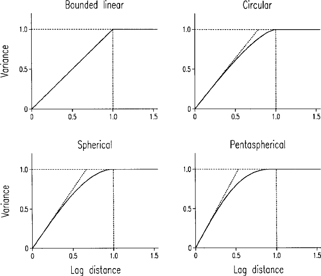
5.2.2 Bounded models

In our experience bounded variation is more common than unbounded variation,

and the variograms have more varied shapes. In most of these models the

variance has a maximum, which is the a priori variance of the process, known in

geostatistics as the sill variance. The variogram may reach its sill at a ﬁnite lag

distance, the range. Alternatively, the variogram may approach its sill asympto-

tically. In some models the semivariance reaches a maximum, only to decrease

again and perhaps ﬂuctuate about its a priori variance. These variograms

represent second-order stationary processes and so have equivalent covariance

functions. They are illustrated in Figures 5.4 and 5.5.

Figure 5.4 Bounded models with ﬁxed ranges: (a) bounded linear; (b) circular;

84 Modelling the Variogram

Bounded linear model

The simplest function for describing bounded variation consists of two straight

lines, as in Figure 5.4(a). The ﬁrst increases and the other has a constant

variance:

gðhÞ¼



for h  a

for h > a;

ð5:13Þ

where c is the sill variance and a is the range. Evidently its slope at the origin is

c=a. It is CNSD in one dimension ðR

Þ only; it may not be used to describe

variation in two and three dimensions.

We can derive the variogram for the bounded linear model heuristically as

follows. We start with a stationary ‘white noise’ process, YðxÞ, in one dimen-

sion, i.e. a random process with random variables at all positions along a line

but in which there is no spatial dependence or autocorrelation. It has a mean m

and variance s

. Suppose that we pass the process through a simple linear ﬁlte r

of ﬁnite length a to obtain

ZðxÞm ¼

xþa

Yðv Þdv: ð5:14Þ

Thus, we average YðxÞ within the interval a to obtain the corresponding ZðxÞ.

Consider now the variable ZðxÞ derived from two segments of the process YðxÞ,

one from x

to x

and the other from x

to x

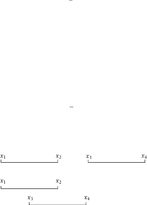
. They may overlap or not, as below.

Evidently, if the two segments do not overlap, as in the upper example, then we

should expect their means in ZðxÞ to be independent. But if they do overlap, as

in the lower example, then they will share some of the original white noise

series; their means will not be independent, and we should expect some

autocorrelation. In general, the closer is x

to x

(and x

to x

) and the longer

is a, the stronger should be the correlation. In fact when x

coincides with x

(and x

with x

) we should have perfect correlation. The only question is what

form the correlation takes as x

approaches x

Authorized Models 85

To answer this we consider the discrete analogue of equation (5.14):

Zðx þ dÞm ¼ l

Yðx þ dÞþl

Yðx þ d þ 1Þþl

Yðx þ d þ 2Þ

þþl

a1

Yðx þ d þ a  1Þ; ð5:15Þ

where the l

; l

; ...; l

a1

are weights, here all equal to 1=a, and d ¼ 1=2a is

half the distance between two successive points in the sequence. All more

distant members, say Yðx þ d þa  1 þ bÞ, of the series carry zero weight.

Suppose that YðxÞ is a white noise process; then ZðxÞ is a moving average

process of order a  1. Further, if the variance of YðxÞ is s

then that of ZðxÞ is

¼ l

þ l

þþl

a1

¼ s

a1

i¼0

¼ s

=a; ð5:16Þ

which is familiar as the variance of a mean. It is also the covariance at lag 0,

Cð0Þ. We now want the covariances for the larger lags. These are obtained

simply by extension from the above equation:

CðhÞ¼s

a1h

i¼0

iþh

¼ s

a  h

: ð5:17Þ

The covariances are in order, for h ¼ 0; 1; 2; ...; a  1; a,

a  0

;

a  1

;

a  2

; ...;

a  a þ 1

;

a  a

Dividing through by the Cð0Þ we obtain the autocorrelations, rðhÞ,as

1; ða  1Þ=a; ða  2Þ=a; ...; ða  a þ 1Þ=a; 0:

In words, the covariance and autocorrelation functions decay linearly with

increasing h until h ¼ a, at which point it is 0. Then the autocorrelation

coefﬁcient at any h is simply equal to the proportion of the ﬁlter that overlaps

when the ﬁlter is translated by h. The variogram is obtained simply from

relation (4.14) by

gðhÞ¼Cð0ÞCðhÞ

¼ s

a  h



¼ c



; ð5:18Þ

since c ¼ s

=a ¼ Cð0Þ.

86 Modelling the Variogram