Webster R., Oliver M.A., Geostatistics for Environmental Scientists

Подождите немного. Документ загружается.

Circular model

The formula for the circular variogram is

gðhÞ¼

c 1 

cos

1



ﬃﬃﬃﬃﬃﬃﬃﬃﬃﬃﬃﬃﬃﬃ

1 

()

for h  a;

c for h > a:

ð5:19Þ

The parameters c and a are again the sill and range. The function curves tightly

as it approaches the range (see Figure 5.4(b)) and its gradient at the origin is

4c=pa.ItisCNSDinR

and R

, but not in R

This model can be derived in a way analogous to that of the bounded linear

model from the area of intersection, A, of two discs of diameter a, the centres of

which are separated by distance h.Mate´rn (1960) did this by considering the

densities with which points are distributed at random by a Poisson process in

two overlapping circles. This area is

A ¼

cos

1





ﬃﬃﬃﬃﬃﬃﬃﬃﬃﬃﬃﬃﬃﬃﬃ

 h

for h  a;

for h > a:

ð5:20Þ

If we express this as a fraction of the area, pa

=4, of one of the circles, in the

same way as we expressed the fraction of the linear ﬁlter that overlapped along

the line above, then we obtain the autocorrelation for the separation:

rðhÞ¼

cos

1





ﬃﬃﬃﬃﬃﬃﬃﬃﬃﬃﬃﬃﬃﬃ

1 

()

for h  a: ð5:21Þ

Then from relation (4.14) the variogram, equation (5.19) above, follows.

Spherical model

By a similar line of reasoning we can derive the three-dimensional analogue of the

circular model to obtain the spherical correlation function and variogram. The

volume of intersection of two spheres of diameter a with their centres h apart is

V ¼

 a

h þ



for h  a;

0 otherwise:

ð5:22Þ

The volume of a sphere is

, and so dividing by it gives the autocorrelation

rðhÞ¼

1 



for h  a;

0 for h > a;

ð5:23Þ

Authorized Models 87

and the variogram is

gðhÞ¼





()

for h  a;

c for h > a:

ð5:24Þ

The spherical model seems the obvious one to describe variation in three-

dimensional bodies of rock, and it has proved well suited to them. It would seem

less obviously suited for describing the variation in one and two dimensions,

which is usually what is needed in soil and land resource survey. Yet it nearly

always ﬁts experimental results from soil sampling better than the one- and

two-dimensional analogues. The function curves more gradually than they do

Figure 5.4(c), and the reason is probably that there are additional sources of

variation at other scales that it can represent. Its gradient at the origin is 3c=2a.

It is CNSD in R

and R

as well as in R

The spherical function is one of the most frequently used models in geostatis-

tics, in one, two and three dimensions. It represents transition features that have

a common extent and which appear as patches, some with large values and

others with small ones. The average diameter of the patches is represented by the

range of the model. One can see this interpretation by simulating a large ﬁeld of

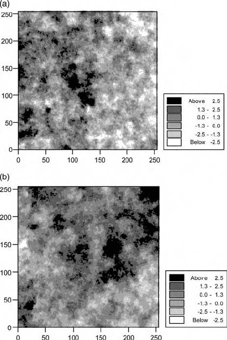
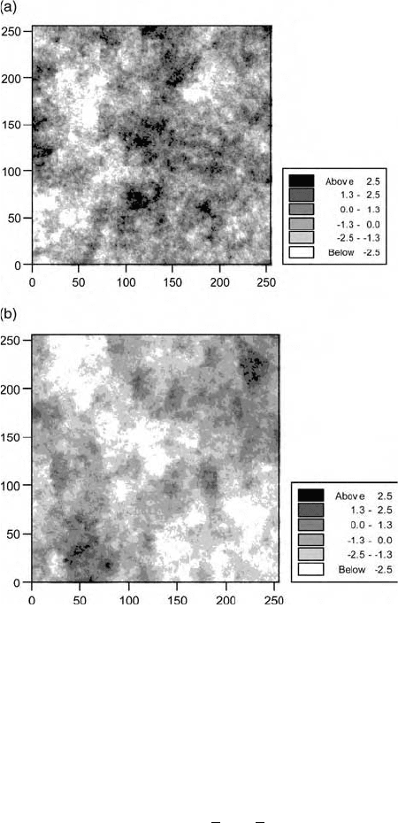
values using the function as the generator. Figures 5.5 and 5.6(a) are examples in

which values have been simulated on a 256 256 square grid with unit interval.

The model had a sill variance, c ¼ 1:0, and ranges of a ¼ 15; 25 and 50 units in

Figures 5.5(a), 5.5(b) and 5.6(a), respectively. The maps show that the extents of

the patches with large and small values increase as the range increases. The

patches have a fairly regular form.

Pentaspherical model

Following Mate´rn (1960), McBratney and Webster (1986) extended the line of

reasoning to obtain the ﬁve-dimensional analogue of the above, the pentasphe-

rical function:

gðhÞ¼





()

for h  a;

c for h > a :

ð5:25Þ

It is useful in that its curve is somewhat more gradual than that of the spherical

model Figure 5.4(d). Its gradient at the origin is 15c=8a. Again it is CNSD in R

and R

Exponential model

A function that is also much used in geostati stics is the negative exponential:

gðhÞ¼c 1  exp 



; ð5:26Þ

88 Modelling the Variogram

with sill c, and a distance parameter, r, that deﬁnes the spatial extent of the

model. The function approaches its sill asymptotically, and so it does not have a

ﬁnite range. Nevertheless, for practical purposes it is convenient to assign it an

effective range, and this is usually taken as the distance at which g equals 95%

of the sill variance, approximately 3r. Its slope at the origin is c=r. Figure 5.7(a)

shows it.

The function has an important place in statistical theory. It represents the

essence of randomness in space. It is the variogram of ﬁrst-order autoregressive

and Markov processes. Its equivalent autocorrelation function has been the

basis of several theoretical studies of the efﬁciency of sampling designs by, for

example, Cochran (1946), Yates (1948), Quenouille (1949) and Mate´rn

(1960). We should expect variograms of this form where differences in soil

Figure 5.5 Simulated ﬁelds of values using spherical functions, equation (5.24), with

distance parameters (a) a ¼ 15, (b) a ¼ 25.

Authorized Models 89

type are the main contributors to soil variation and where the boundaries

between types occur at random as a Poisson process. Burgess and Webster

(1984) found this to be the situation in many instances. If the intensity of the

process is h then the mean distance between bou ndaries is



d ¼ 1=h and the

variogram is

gðhÞ¼cf1  expðh=



dÞg

¼ cf1  expðhhÞg:

ð5:27Þ

Put another way, this is the variogram of a transition process in which the

structures have random extents.

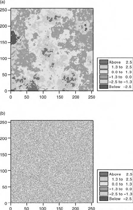
Figure 5.6 Simulated ﬁelds of values using: (a) a spherical function, equation (5.24),

with distance parameter a ¼ 50; (b) a pure nugget variogram, equation (5.33).

90 Modelling the Variogram

Simulated ﬁelds obtained from an exponential function with an asymptote

approaching 1.0 and distance parameters, r, of 5 and 16 are shown in

Figure 5.8(a) and 5.8(b), respectively. The patches of large and small values

in the two ﬁelds are similarly irregular, but the average sizes of the patches

show the different spatial scales of the generator.

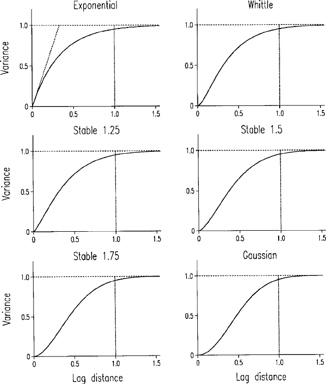
Figure 5.7 Models with asymptotic bounds. All are scaled so that the effective range

where the function reaches 0.95 of its sill is approximately 1, marked by the vertical lines

on the graphs. (a) a ¼ 1 (exponential), r ¼ 0:333; (b) Whittle, r ¼ 0:25; (c) a ¼ 1:25

(stable), r ¼ 0:416; (d) a ¼ 1: 5 (stable), r ¼ 0:478; (e) a ¼ 1:75 (stable), r ¼ 0:533; (f)

a ¼ 2 (Gaussian), r ¼ 1=

ﬃﬃﬃ

Authorized Models 91

Whittle’s elementary correlation

Whittle (1954) showed that a simple stochastic diffusion process also has an

exponential variogram in one and three dimensions. In R

, however, the

process leads to Whittle’s elementary correlation, given by

gðhÞ¼c 1 



: ð5:28Þ

The parameter c is the sill, as before, the a priori variance of the process, r is a

distance parameter, and K

is the modiﬁed Bessel function of the second

kind. Like the exponential function, Whittle’s function approaches its sill

Figure 5.8 Simulated ﬁelds of values from exponential functions (equation (5.26)),

with distance parameters (a) r ¼ 5, (b) r ¼ 16.

92 Modelling the Variogram

asymptotically and so has no deﬁnite range. Its effective range may be chosen

as for the exponential function where the semivariance reaches 95% of the sill,

and this is at approximately 4r. The function approaches the origin with a

decreasing gradient, however, and appears slightly sigmoid when plotted,

Figure 5.7(b).

Gaussian model

Another function with reverse curvature near the origin recurs again and again

in geostatistical texts and software packages. It is the so-called Gaussian mod el

(Figure 5.7(f)) with equation

gðhÞ¼c 1  exp 



: ð5:29Þ

Once more, c is the sill and r is a distance parameter. The function approaches

its sill asymptotically, and it can be rega rded as having an effective range of

approximately

ﬃﬃﬃ

r where it reaches 95% of its sill variance.

A seri ous disadvantage of the model is that it approaches the origin with zero

gradient, which we saw above as the limit for random variation and at which

the underlying variation becomes continuous and twice differentiable. This can

lead to unstable kriging equations, which we present in Chapter 8, and bizarre

effects when used for estimation—see Wackernagel (2003) for examples.

In general we deprecate this model. If a variogram appears somewhat

sigmoid then we recommend the theoretically attractive Whittle function.

Alternatively, if the reverse curvature is stronger you may replace the exponent

2 in equation (5.29) by an additional parameter, say a, with a value less

than 2:

gðhÞ¼c 1  exp 



: ð5:30Þ

Wackernagel (2003) calls these ‘stable models’. Some examples of them are

shown in Figure 5.7(c)–(e) with various values of a, and we have used the model

with a ¼ 1:965 to describe topographic variation (Webster and Oliver, 2006).

Cubic model

Another bounded model with reverse curvature near the origin is the cubic

function. Its formul a is

gðhÞ¼

c 7



8:75



þ3:5



0:75



()

for h a;

c for h > a:

ð5:31Þ

Authorized Models 93

The parameter a is a ﬁnite range which is approached much more gradually

than in the spherical and pentaspherical models.

There are other simple models used in particular disciplines because of their

theoretical attractions. Examples include the prismato-gravimetric and prismato-

magnetic functions developed in geophysics to model gravimetric and magnetic

anomalies (see Armstrong, 1998). If you work in such a special ﬁeld then you

should ask whether there are preferred functions for the particular applications.

Mate´rn functio n

The Matere´n function is a generalization of several of the functions mentioned

above and so appears attractive for this reason. Its formula is

gðhÞ¼c 1 

n1

GðnÞ





: ð5:32Þ

As in the exponential, Whittle and Gaussian models the function has a distance

parameter r, and c is the sill. It also has a smoothness parameter, n, analogous

to a in the stable models (equation (5.30)), though whereas a is limited to

between 0 and 2, n can vary in the range 0 (very rough) to inﬁnity (very

smooth). It includes the special cases of exponential when n ¼ 0:5 and Whittle’s

function when n ¼ 1. Figure 5.9 shows variograms for several values of n.

Figure 5.9 The Mate´rn function (5.32) with a priori variance c ¼ 1 and distance

parameter r ¼ 20 and ﬁve values of the smoothness parameter n, giving the ﬁve curves.

The curve with n ¼ 0:5 is the exponential and that with n ¼ 1 is Whittle’s function.

After Minasny and McBratney (2005).

94 Modelling the Variogram

Unfortunately, when Minasny and McBratney (2005) examined its potential

for describing soil properties they had difﬁculty ﬁtting it to experimental

variograms. They found that n was poorly estimated by the usual method of

weighted least squares (see below).

Pure nugget

Although the limiting value 0 of the exponent of equation (5.10) for the power

function was excluded because it would give a con stant variance, we do need

some way of expressing such a constant because that is what appears in

practice. We do so by deﬁning a ‘pure nugget’ variogra m as follows:

gðhÞ¼c

f1  dðhÞg; ð5:33Þ

where c

is the variance of the process, and dðhÞ is the Kronecker d which takes

the value 1 when h ¼ 0 and is zero otherwise. If the variable is continuous, as

almost all properties of the soil and natural environment are, then a variogram

that appears as pure nugget has almost certainly failed to detect the spatially

correlated variation because the sampling interval was greater than the scale of

spatial variation.

Since the nugget variance is constant for all h; jhj > 0, it is usually denoted

simply by the variance c

. Figure 5.6(b) shows the simulated ﬁeld from a pure

nugget variogra m. There is no detectable pattern in the variation as there is in

Figures 5.5, 5.6(a) and 5.8.

5.3 COMBINING MODELS

As is apparent in Figures 5.3 , 5.4 and 5.7, all the above functions have simple

shapes. In many instances, however, especially where we have many data,

variograms appear more complex, and we may therefore seek more complex

functions to describe them. The best way to do this is to combine two or more

simple models. Any combination of CNSD functions is itself CNSD. Do not look

for complex mathematical solutions the properties of which are unknown.

The most common requirement is for a model that has a nugget component

in addition to an increasing, or structured, portion. So, for example, the

equation for an exponential variogram with a nugget may be written as

gðhÞ¼c

þ c 1  exp 



; ð5:34Þ

and an example is shown in Figure 5.10(a). Figure 5.11 shows the simulated

ﬁelds for an exponential variogram with parameters c

¼ 0:333, c ¼ 0:667 and

distance parameters, r, of 5 and 16 as before. The speckled appearance within

the patches is the result of the nugget variance.

Combining Models 95

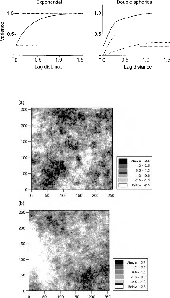
Figure 5.10. Combined (nested) models: (a) single exponential with sill 0.75 plus a

nugget variance of 0.25; (b) double spherical with ranges 0.35 and 1.25 and correspond-

ing sills 0.3 and 0.5 plus a nugget variance of 0.2 with the components shown separately.

Figure 5.11 Simulated ﬁelds of values from exponential functions with nugget variance

one-third of the total variance, equation (5.34): with distance parameters (a) r ¼ 5;

(b) r ¼ 16.

96 Modelling the Variogram