Webster R., Oliver M.A., Geostatistics for Environmental Scientists

Подождите немного. Документ загружается.

skewness increases, the nugget and sill variances increase markedly. The

nugget:sill ratios increase as skewness increases, even though the ﬁelds were

generated by a variogram function with zero nugget. The size of ﬁeld has far less

effect than that observed where asymmetry was caused by a long tail in the

distribution, as in Figure 6.2. For skewness coefﬁcients up to 1.5 the variograms

tend to retain their shape, but for g

¼ 3:0 (not shown) the variograms were

almost pure nugget. Variograms computed from ﬁelds with aggregated outliers

are very different from those where the outliers were randomly located.

Figure 6.5(a) shows the variograms computed from the ﬁelds on a 10 m grid

(400 values) with outliers aggregated near the edge and for several coefﬁcients of

skewness. The nugget variances are close to zero, but the sill variances increase

with increasing skewness. Nevertheless, these sill variances are less than those for

the randomly located outliers, Figure 6.4(b). For outliers grouped near the centres

of the ﬁelds on the 10-m grid, shown in Figure 6.5(b), the variograms have small

or zero nugget variances. The sill variances, however, increase more with

increasing skewness than do those in Figure 6.5(a); they are more similar to

those for the randomly located outliers, Figure 6.4(b).

Kerry and Oliver (2007b) transformed the data to square roots and loga-

rithms, but these transformations were not as effective in dealing with the

observed effects of the outliers as the robust variogram estimators. Figure 6.6(a)

shows that Matheron’s method-of-moments estimator and the three robust

estimators described above result in similar experimental variograms for the

normal ﬁeld. The met hod-of-moments variogram is closest to the generating

Figure 6.5 Experimental variograms (shown by point symbols) computed from ﬁelds

of 400 points (10-m grid) contaminated by spatially aggregated outliers (a) at the edges;

(b) at the centre of ﬁelds, and for ﬁve coefﬁcients of skewness. The solid lines represent

the spherical generating function.

Reliability of the Experimental Variogram 117

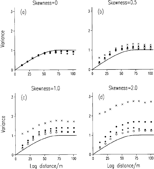
model, however. Figure 6.6(b)–(d) shows that as skewness increases Mather-

on’s variogram departs much more from the generating function than the

robust variograms. Of the latter, Dowd’s and Genton’s variograms remain closer

to the original model than does that of Cressie and Hawkins.

Kerry and Oliver (2007b) concluded from their results that skewness caused

by outliers must be dealt with regardless of the number of data. Furthermore,

the results suggested practitioners should act when the skewness, g

, exceeds

0.5. Robust estimators provide a solution, but they did not perform equally well

in all the situations examined. The current ‘best practice’ approach of removing

outliers before computing the variogram appears to be the most appropriate

where they are randomly located and will not be returned to the data for

kriging. However, where outliers are crucial in an investigation, as on

contaminated sites, practitioners should compute several robust variograms

and compare them by cross-validation (see Chapter 8).

Figure 6.6 Experimental variograms computed by Matheron’s method-of-moments

estimator () and Cressie and Hawkins’s (), Dowd’s () and Genton’s (?) robust

estimators from ﬁelds of 400 points (10-m grid) with skewness coefﬁcients of (a) 0,

(b) 1.0, (c) 1.5, (d) 2.0, caused by randomly located outliers. The solid lines are of the

spherical generating function.

118 Reliability of the Experimental Variogram and Nested Sampling

6.1.2 Sample size and design

The reliability of the experimental variogram is affected not only by the

statistical distribution of the data but also by the size of the sample (or its

inverse, the density of data), and the conﬁguration or design of the sample.

Hundreds, if not thousands, of experimental variograms are now displayed in

published papers, reports, theses and books. The y are derived from samples of as

few as 24 individual measurements up to several tho usands, though typically

they are computed from 100–200 data. Those based on fewer than 50 data are

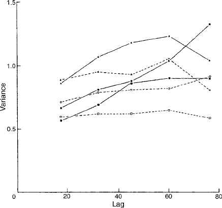
often erratic sequences of experimental values with little or no evident

structure. Figure 6.7 shows some examples. As the size of sample is increased

such scatter decreases and the form of the variogram becomes clearer: the

plotted points tend to be closer to an increasing line . Evidently the larger is the

sample from which the variogram is computed the more precisely it is

estimated. In most instances, however, the precision is unknown, and we

cannot determine how large a sample to take to achieve some desired precision.

The classical formulae for determining conﬁdence intervals cannot be applied

unless the sampling itself is designed for the purpose, as suggested by Brus and

de Gruijter (1994). Practitioners who attempt to assign error to their estimates

based on these formulae are misguided. There are several reasons why:

(i) the same data are used more than once in each estimate;

(ii) the estimates are correlated;

(iii) the sampling is not sufﬁciently ran domized.

Figure 6.7 Graphs of sample variograms with 49 data. Reproduced with permission

Journal of Soil Science, Vol. 43, # Blackwell Publishing.

Reliability of the Experimental Variogram 119

Before we proceed further we must be clear which variogram we are

attempting to estimate from the experimental one. In Chapter 4 we identiﬁed

two distinct functions, one the theoretical variogra m and the other the local or

regional variogram. The ﬁrst is the variogram of the underlying stochastic

process, whereas the local variogram is that of the particular realization in the

region and called the non-ergodic variogram by Brus and de Gruijter (1994).

An experimental vari ogram may contain error deriving from different realiza-

tions of the random function or from different samples of the particular

realization, or both. In the ﬁrst case the error arises from ﬂuctuation in the

generator, whereas in the second the error arises from the sampling. We take

the view here that for most practical purposes we are concerned with just one

realization in the region, so we should try to estimate the sampling error

expressed in the estimation variance or conﬁdence limits.

Matheron (1965) gave a formula to provide a ﬁrst approximation to the

estimation variances of the local variogram:

var½

ðhÞ 

4gðhÞs

; ð6:5Þ

where gðhÞ is the value of the theoretical variogram at lag h;

ðhÞ is the

estimate of the regional semivariance at that lag, and s

is the total variance

in the region, i.e. the dispersion variance . Matheron de scribe s N

as the

number of points effectively used, i. e. t he number of points th at are super-

posed in t he intersecti on of the re gion with itself when translated by the

vector h. For a regular transect of length M it is the number of paired

comparisons (M  h) con tributi ng to the estimate of g

ðhÞ.Itisfromthisthat

confusion has arisen about the number o f observatio ns needed to estimate

the vario gram r eliably and in particular a s uggest ed mi nimum of 30–50

paired comparisons for any one

ðhÞ (Journel and Huijbregts, 197 8). T he

advice seems to have been intended for one dimension, but unfortunately it

has been applied widely in two dimensions and has given practitioners a false

sense of secu rity when compu ting variogram s from small samples.

Mun˜ oz-Pardo (1987) pursued Matheron’s idea for estimating the estimation

variances for variograms with a sill (bounded). He derived the following

expression for the estimation variance of a semivariance:

var½

ðhÞ ¼

f ðx; y; hÞdxdy þ

ðhÞ

i¼1

ðhÞ

j¼1

f ðx

; x

; hÞ



ðhÞS

ðhÞ

i¼1

f ðx

; x; hÞdx;

ð6:6Þ

120 Reliability of the Experimental Variogram and Nested Sampling

where

f ðx; y; hÞ¼fgðx  y þ hÞþgðx  y  hÞ2gðx  yÞg

ð6:7Þ

for any value of i and j.Inequation(6.6)

ðhÞ denotes the estimated value of the

regional variogram at lag h; S

is the area of intersection when the region is

translated by the vector h; N

is the number of sampling points in the intersection,

and x and y are two points that describe the region independently. Mun˜oz-Pardo

solved the equation by numerical integration. He showed that the estimation

variance depended on the effective range of the variogram in relation to the size of

the region as well as on the size of the sample.

One way of obtaining conﬁdence limits on variograms is by Monte Carlo

methods (Webster and Oliver, 1992). There are two possible approaches,

depending on which variogram (theoretical or regi onal) we are concerned

with. If it is the ﬁrst then one simulates many realizations from a particular

model and computes the experimental variogram of each, as did McBratney and

Webster (1986), Taylor and Burrough (1986) and Shafer and Varljen (1990).

The result will show the ﬂuctuation arising from the gen erator, and the

quantiles of the obse rved values for each lag would be reasonable estimates

of the conﬁdence intervals for new realizations.

Environmental scientists are more often concerned with single particular

realizations, which they must sample, and so they are interested in the

sampling ﬂuctuation. Here the Monte Carlo approach is to generate a

single large ﬁeld of ‘data’ from a plausible model of the variation in the region,

sample repeatedly from it, and for each sample compute the sample variogram.

The variation in the variograms thereby obtained will be sampling ﬂuctuation,

and the quanti les of the semivariances may be used as conﬁdence limits on the

regional variogram.

Webster and Oliver (1992) expl ored this approach by simulating large

autocorrelated random ﬁelds, which they then sampled on grids and transects

of varying size and density with random starting points. We illustrate the

approach here with one of their examples.

A ﬁeld of 65 536 random values on a 256  256 square grid with unit

interval was generated by sequential Gaussian simulation (Deutsch and Journel,

1992) and an exponential variogram (equation (5.26) ) with distance para-

meter r ¼ 16 units. It is displayed in Figure 5.8(b). We can imagine it as one of

exchangeable K in the soil. There are distinct patches with large and small

values showing that spatial dependence extends on average to about 50 units,

which is about 3 times the distance parameter (as explained in Chapter 5). The

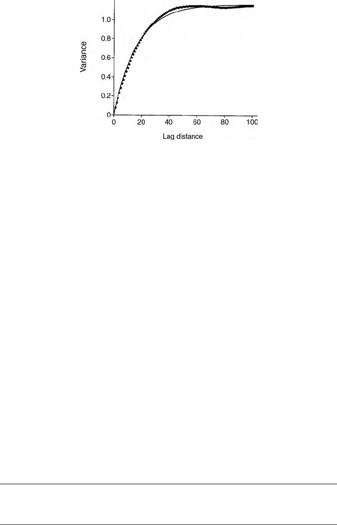
variogram from the exhaustive data is close to the generating function (Figure

6.8). The ﬁeld was then sampled on regular square grid s with the sample sizes

and sampling intervals in Table 6.3. No position was used more than once, and

so no comparisons were duplicated.

Reliability of the Experimental Variogram 121

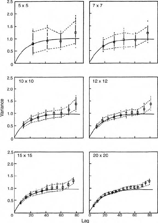
We computed the variograms for all the samples, and in Figure 6.9 we plot

the results on the same set of axes. The variograms of the samples of 25

show the wide spread of estimates around the variogram of the generating

function. The dotted lines are the 90th percent iles, i.e. the symmetrical 90%

conﬁdence limits. The other graphs in the sequence show how the conﬁdence

intervals narrow as the size of the sample increases. A sample of 100 points

appears to give moderate conﬁdence, but to attain satisfaction at leas t 144

measurements seem necessary. Increasing the sample to 225 points provides

rather little improvement, whereas 400 data enable the variogram to be

estimated with great precision.

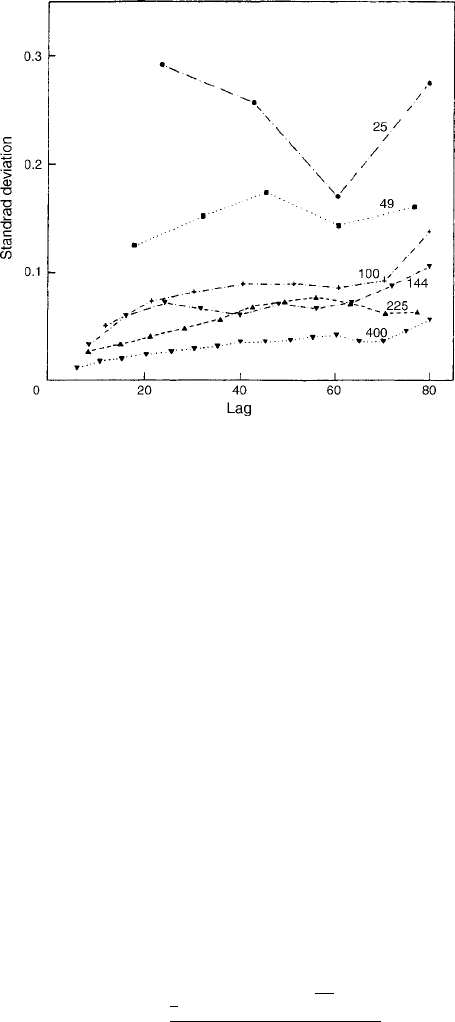
The results can be summarized in a graph of the standard deviation of the

observed semivariances against the size of the sam ple (Figure 6.10). The

standard deviation decreases, and the 90th percentiles narrow, with increasing

sample size. We can also judge from Figure 6.10 approximately what size of

sample to use to achieve some particular conﬁdence.

The results show clearly that sample variograms from only 25 and 49 data

have wide conﬁdence intervals, and are therefore imprecise. Samples of 100

might be acceptable in some circumstances, and one s of 144 are likely to be

adequate, at least with nor mally distributed isotropic data as in the generated

ﬁelds. Variograms computed from samples of 225 will almost certainly be

reliable, and samples of 400 seem extravagant. Based on this evidence we

recommend that you have no fewer than 100 sampling points and ideally 150

to estimate the variogra m reliably in two dimensions if the variation is isotropic.

Figure 6.8 The exhaustive variogram computed from Figure 5.5(a).

Table 6.3 Sample size, spacing and number of iterations.

Size 25 49 199 144 225 400

Interval 20 15 10 8 7 5

Iterations 100 100 100 64 49 25

122 Reliability of the Experimental Variogram and Nested Sampling

For anisotropic variation we recommend at least 250 sample points because of

the nee d to compute variograms in several directions.

The results also show the importance of interpreting N

of equation (6.5)

correctly. Forty-nine points on a square grid gave us 84–240 paired compar-

isons, which would have seemed more than enough against the 30–50

comparisons regarded by some authorities as adequate. With 100 points there

were 180–774 comparisons, and still the variograms were somewhat erratic.

Figure 6.9 Semivariances computed on samples of various sizes from Figure 5.5(a)

and 90% conﬁdence limits obtained. Reproduced with permission Journal of Soil Science,

Vol. 43, # Blackwell Publishing.

Reliability of the Experimental Variogram 123

Brus and de Gruijter (1994) viewed the problem differently. They pointed out

that until you know the variogram accurately you cannot simulate realistic

ﬁelds of values from which to sample. If the variogram used for the simulation

has been estimated from few data then the realization gen erated might

represent the true situation in the region poorly and lead to misleading

conﬁdence limits. They proposed a procedure based on classical sampling

theory. For each lag, h, they repeatedly selected pairs of points, the ﬁrst of

each pair at random and the second determined by h. In the simplest design,

simple random sampling (Chapter 2), the ﬁrst point is chosen without regard to

any other, and all points have an equal chance of inclusion. If the variation is

isotropic then the second poin t can be chosen at distance h ¼jhj from the ﬁrst

but in a random direction. The mean of the individual squared differences

obtained with equation (4.40),

gðhÞ, is an unbiased estimate of gðhÞ.

Since the pairs of points are chosen independently of one another the

calculated squared differences are independent, and so the sampling variance

gðhÞ can be estimated by the classical formula. If we denote the squared

difference at lag h by d

ðhÞ then, following Cochran (1977), we can write the

variance of the semivariance as

var½

gðhÞ ¼ var½0:5d

ðhÞ=mðhÞ

mðhÞ

i¼1

ðhÞd

ðhÞg

mðhÞfmðhÞ1g

; ð6:8Þ

Figure 6.10 Standard deviations of semivariances for the several grid samplings from

Figure 5.5(a). Reproduced with permission Journal of Soil Science, Vol. 43, # Blackwell

Publishing.

124 Reliability of the Experimental Variogram and Nested Sampling

where d

ðhÞ is the mean of the squared difference at lag h . Further, choosing

fresh pairs of points for each h or h provides independent estimates for the

different lags.

As we saw in Chapter 2, simple random sampling is inefﬁcient, and the precision

orefﬁciencycanbe improvedby betterdesign.BrusanddeGruijter(1994)elaborate

theprocedurefor stratiﬁed sampling andgive the formulae forthe estimatorand the

estimation variance. The formulae can be modiﬁed for other designs.

The estimation variance has still to be convert ed into conﬁdence limits, and

for this one must assume a distribution. It is not immediately evident what that

distribution should be. One might expect the individual d

ðhÞ to be distributed

as x

. Their means, however, are likely to approach normality with increasing

mðhÞ in accordance with the cen tral limit theorem. Brus and de Gruijter

calculated limits on this assumption but found that it was not entirely

satisfactory for the fairly small mðhÞ in their study: they obta ined several

negative lower limits at the 90% level, suggesting that the conﬁdence interval is

not symmetric, at least for the small samples they took. This contrasts with our

ﬁnding, with larger samples, that limits were approximately symmetrical.

Despite this weakness, the method proposed by Brus and de Gruijter gives sound

unbiased estimates of the sampling variance of gðhÞ, but large samples are needed

to obtain precise estimates. In addition, the sampling scheme with pairs of points

scatteredirregularly and unevenly is inefﬁcient for subsequent kriging (Chapter 8).

Although the above approaches to the problem differ, both sho w that the

conﬁdence intervals are very wide with small samples: you need a large sample

to estimate the variogram by Matheron’s method of moments reliably.

Pardo-Igu´zquiza (1998) suggested that ‘a few dozen data may sufﬁce’ to

estimate variogram parameters by residual maximum likelihood (REML) because

of the efﬁciency of the method; see Section 9.2 for more detail. In this approach

the model parameters are estimated directly from the generalized increments of a

covariance matrix of the full data. As a consequence there is no smoothing of the

spatial structure because there is no ad hoc deﬁnition of lag classes. Kerry and

Oliver (2007c) compared variograms computed by the method of moments and

REML as described by Pardo-Igu´zquiza (1997) for various numbers of empirical

data. Their results show that where there are fewer than 100 data, but more than

50, the REML variograms gave more accurate predictions as assesed by cross-

validation (see Chapter 8) than did the method-of-moments variograms. Never-

theless, even with REML variograms the accuracy of prediction decreased when

there were fewer than 100 sites, and practitioners should still aim for at least 100

data for accurate predictions.

Practitioners might wonder why computing variograms by REML is not a

standard approach. There are several drawbacks to the method:

 the nee d for second-order stationarity;

 the very limited range of variogram functions that can be ﬁtted by the

readily available software;

Reliability of the Experimental Variogram 125

 it is computationally intensive;

 the limitations to the methods for maximizing the log-likelihood function—

see equation (9.25) .

In spite of these, Kerry and Oliver (2007c) concluded that the REML variogram

is valuable where it is impractical to obtain as many as 100 data.

6.1.3 Sample spacing

In general, as the size of sample increases so the spacing between sampling

points decreas es for a given region. Nevertheless, we cannot simply allow the

sample spacing to be dictated by the size of sample. The spacing must relate to

the scale or scales of variation in the region. Otherwise we might sample too

sparsely to identify correlation. We should therefore know roughly the spatial

scale of variation in Z so as to choose a sensible sampling density.

Some variables, such as vegetation, have visible patterns, and their

spatial scales are obvious. Many properties of soil, rocks, atmosphere and water,

on the other hand, are invisible, and so one cannot judge the spatial scales on

which they vary without ﬁrst sampling. They can also vary on scales that differ

by several orders of magnitude simultaneously, as described in Chapter 4. In some

instances an approximate scale of variation can be judged from that of other

features, such as landform or vegetation, but often it is more elusive.

Let us consider the following situations.

1. Terra incognita. If we know nothing of the pattern or scale of the variation

then it is difﬁcult to choose a sampling interval rationally. A large interval

might be too large to capture the autocorrelation. If we choose a small

interval then we might have to restrict the area sampled to stay within a

budget and fail to estimate long-range variation. If we were to sample a

whole region densely and the variation turned out to be entirely long-range

then we should have wasted money tryi ng to estimate short-range varia-

tion. We want some means of estimating, even roughly, the spatial scale of

variation effectively and economically.

2. We have data from a previous survey, but their experimental vario-

gram(s) seem(s) ﬂat, or pure nugget, i.e. there is no evident spatial

correlat ion. If the va ria bles are continuous then we ca n assume that

the correlation range is less than the smallest sampling interval. We can

know no m ore than that .

3. We have variograms with apparent ‘structure’, but feel that some parts of

the region are undersampled and others oversampled, and that some

sampling points could be positioned more effectively to optimize estimation.

The problems faced in 1 and 2 can be resolved by starting with a nested survey

and analysis, which we now describe.

126 Reliability of the Experimental Variogram and Nested Sampling