Webster R., Oliver M.A., Geostatistics for Environmental Scientists

Подождите немного. Документ загружается.

6.2 THEORY OF NESTED SAMPLING AND ANALYSIS

The model of nested variation is based on the notion that a population can be

divided into classes at two or more categoric levels in a hierarchy. The

population can then be sampled with a multi-stage (multi-level) or nested

scheme to estimate the variance at each level. The population is divided initially

into classes at stage 1, and these are subdivided at stage 2 into subclasses,

which in turn can be subdivided further at stage 3 to give ﬁner classes, and so

on, to form a nested or hierarchical classiﬁcation with m stages. In each case

the class at the lower level is contained completely within the one immediately

above it, and each sampling point is contained in one and only one class at each

and ever y level. The system is a strict hierarchy, and a single observation

embodies variation contributed by each of the stages, including an unresolved

variance within the classes at the ﬁnest level of resolution. We can estimate

these contributions to the variance by a hierarchical analysis of variance

(ANOVA).

Youden and Mehlich (1937) saw that for an attribute distributed in space the

stages could be represented by a hierarchy corresponding to different distances.

They adapted classical multi-stage sampling so that each stage in the hierarchy

represented a distance between sampling points. They sampled at random, with

only the distances between pairs ﬁxed, and so the random effects model, model

II of Marcuse (1949), is appropriate for the ANOVA.

For a design with m stages the data are modelled as

ijk...m

¼ m þ A

þ B

þþ"

ijk...m

; ð6:9Þ

where Z

ijk...m

is the value of the mth unit in ..., in the kth class at stage 3, in the

jth class at stage 2, and in the ith class at stage 1. The general mean is m; A

the difference between m and the mean of class i in the ﬁrst category; B

is the

difference between the mean of the jth subclass in class i and the mean of class i;

and so on. The ﬁnal quantity "

ijk...m

represents the deviation of the obse rved

value from its class mean at the last stage of subdivision. The quantities

; B

; C

ijk

; ...;"

ijk...m

are assumed to be independent random variables asso-

ciated with stages 1; 2; 3; ...; m, respectively, having means of zero and

variances s

; s

; ...; s

. The latter are the compon ents of variance for

the respective stages. They are estimated according to the scheme in Table 6.4.

The quantities n

; n

; ...; n

, in the table are the numbers of subdivisions of

each class at the several levels. If for each stage, say j, n

is constant then the

design is balanced. All the n

; j ¼ 1; 2; ...; n

, are known for any particular

design, and so we can dete rmine the components of variance for all stages in

the classiﬁcation and the residual variance from the right-hand column of

Table 6.4.

Theory of Nested Sampling and Analysis 127

The individual component for a given stage measures the variation attribu-

table to that stage, and together they sum to the total variance:

¼ s

þ s

þþs

: ð6:10Þ

The components of variance for each spacing from this analysis reveal over what

part of the spatial scale most of the variation occurs. The particular merit of the

method is that a wide range of spatial scales can be covered in a single analysis.

6.2.1 Link with regionalized variable theory

Although the hierarchical ANOVA derives from classical statistics, Miesch

(1975) showed its links with geostatistics. He also showed that it can provide

a ﬁrst approximation to the vari ogram if the components of variance are

accumulated, starting with the smallest spacing. For the m stages of subdivision

we have the corresponding distances d

; d

m1

; ...; d

, where d

is the sho rtest

distance at the mth stage and d

is the largest distance at the ﬁrst stage. Then

the equivalence is given by

¼ gðd

Þ;

m1

þ s

¼ gðd

m1

Þ;

m2

þ s

m1

þ s

¼ gðd

m2

Þ;

ð6:11Þ

and so on. In practice, the distances are chosen in geometric progression in

which each is at least 3 times the previous one; in this way the branches of the

hierarchy do not overlap on the ground, and it is clear to which each sampling

belongs at every stage. The components tend to be fairly imprecise estimates of

the true semivariances because each is usually based on few degrees of freedom,

at least in the ﬁrst few stages. We should also bear in mind that they are not

Table 6.4 Hierarchical analysis of variance: parameters estimated.

Source Degrees of freedom Parameters estimated

Stage 1 n

 1 s

þ n

m1

þþn

m1

...n

þn

m1

...n

Stage 2 n

ðn

 1Þ s

þ n

m1

þþn

m1

...n

Stage 3 n

ðn

 1Þ s

þ n

m1

þþn

m1

...n

Stage m  1 n

...ðn

m1

 1Þ s

þ n

m1

Stage m(residual) n

...n

m1

ðn

 1Þ s

Total n

...n

m1

 1

128 Reliability of the Experimental Variogram and Nested Sampling

entirely independent of one another and that variation in different directions

cannot be distinguis hed.

The values gðd

Þ are the equivalent semivariances. When plotted against

distance they provide a ﬁrst appr oximation to the variogram. The result might

be rough, but it indicates how Z varies in space in the region over several orders

of magnitude of distance in a single analysis and with modest sampling. For this

reason it is ideal for reconnaissance where little or nothing is known. Once the

spatial scale is known then a subsequent survey can be planned to estimate the

variogram precisely (Oliver and Webster, 1986) or to plan a more general

survey over a larger area. Alternatively, the analysis might show that all the

variation occurs over very short distances, and that attempting to measure

spatial correlation and map the variable(s) is pointless or would be too costly.

6.2.2 Case study: Youden and Mehlich’s survey

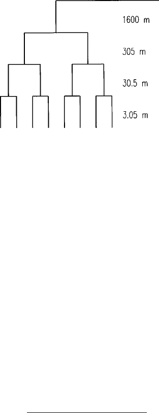
We illustrate the technique with an example from Youden and Mehlich’s

(1937) original paper. The authors’ sampling scheme to survey the soil in

Broome County in New York State had four stages (Table 6.5). They applied it

to two soil series: the Culvers and the Sassafras. On each soil type they selected

nine primary centres 1.6 km apart forming level 1 in the hierarchy. At the next

level (level 2) one subcentre was selected 305 m away from each of the main

centres (18 locations). At level 3 two sampling points were chosen 30.5 m from

the mai n centre and the subcentre (36 locations). At level 4 each site was

replicated with ano ther 3.05 m away, to give 72 sampling poin ts in all. The

survey was fully balanced, so that all classes at a particular level were

subdivided equally to form the hierarchy (Figure 6.11). The progression of

the sampling intervals was geometric, as above, with a 10-fold multiplication of

the distances except at the highest level. As a result the authors felt able to

regard the components of variance as independent, thereby allowing conﬁdence

intervals to be determined. At each sampling point the pH was determined on

soil take n from a depth of 0–15 cm.

Table 6.5 Components of variance of pH in two soil series sampled by Youden and

Mehlich (1937).

Culvers series 0–15 cm Sassafras series 0–15 cm

Degrees of Estimated Percentage Estimated Percentage

Stage Spacing/m freedom component of variance component of variance

1 1600.0 8 0.02819 39.7 0 0

2 305.0 9 0.02340 32.9 0.04440 60.3

3 30.5 18 0.00552 7.8 0.00698 9.8

4 3.05 36 0.01391 19.6 0.02225 30.2

Theory of Nested Sampling and Analysis 129

For each soil series the variation associated with each sampling interval was

determined by a nested ANOVA as in Table 6.4. First the sums of squares of the

deviations of the means of the classes at level 1 from the general mean were

computed, and then each was multiplied by the number of observations that

made up the class mean. For each class at level 2, the difference between its

mean and the mean of the class to which it belongs in level 1 was squared and

multiplied by the number of observations in that class. The sum of these values

is the appropriate sum of squares. This was repeated for each stage, and the

sums of squares of the individual levels sum to the total sum of squares . The

mean squares were obtained by dividing the sums of squares of each stage by

the appropriate degrees of freedom (Table 6.4). The mean square at each level,

apart from the lowest, contains a unique contribution to the variance from that

level, plus contributions from the components at all levels below (Table 6.4).

For instance, the unique contrib ution to the variance at level 2 (Table 6.4) is

m1

...n

. This enables each component to be determined separately from

its mea n square. For a balanced design the value of each component can be

tested to judge whether it is larger than zero by the F ratio:

F ¼

mean square at level m

mean square at leve l m þ 1

: ð6:12Þ

Table 6.5 gives the results of the analysis. The components of variance can

now be accumulated, starting with that for the lowest level, and plotted against

sample spacing (Figure 6.12). This gives a ﬁrst approximation to the variogram,

a reconnaissance variogram. Figure 6.12 shows the accumulated components

of variance for the Culvers and Sassafras series plotted against distance on a

logarithmic scale. The variance for the Culvers series increases substantially as

the distance between sampling points increases and without limit (unbounded).

The sample variance for the Sassafras series does reach a maximum (bounded),

Figure 6.11 Topological structure of the balanced nested sampling design of Youden

and Mehlich (1937).

130 Reliability of the Experimental Variogram and Nested Sampling

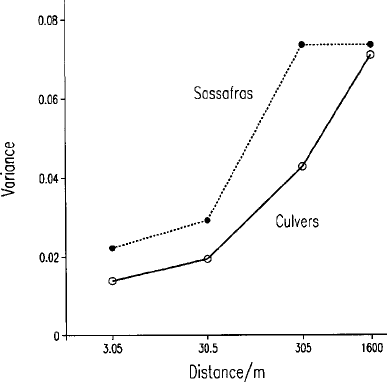
and we might therefore treat the variation as second-order stationary. If we

project the variances to spacings less than the smallest, 3 m, then both seem to

approach limits larger than 0. Such limits are examples of what we now

recognize as nugget variance.

6.2.3 Unequal sampling

The sampling designs described above are fully balanced in the sense tha t all

classes at each particular stage are subdivi ded equally. For the particular design

in Broome County the sample size doubles with each additional stage in the

hierarchy after the ﬁrst. To achieve good spatial resolution might require many

stages and result in prohibitively expensive sampling for reconnaissance. It

would to some extent defeat the object whereby one is trying to obtain

preliminary information for modest effort. As it happens, full replication at

each stage is unnecessary because the mean squares for the lower stages are

estimated more precisely than those for the higher ones. Economy can be

achieved by replicating only a proportion of the sampling centres in the lower

stages. Oliver and Webster (1986) used ﬁve stages, but in more recent

applications, Webster and Boag (1992), Badr et al. (1993) and Oliver and

Badr (1995) have used seven. The resulting schemes are unbalanced, and this

makes estimating the components somewhat more complex because the

Figure 6.12 Variograms of pH from Youden and Mehlich’s surveys of pH in Culvers

and Sassafras soil series by accumulation of the components of variance. Note the

logarithmic scale for distance on the abscissa.

Theory of Nested Sampling and Analysis 131

coefﬁcients of the components are no longer simple multiples of the number of

divisions in the levels as they are in Table 6.4, which must be replaced by a

table such as Table 6.6 for a sample of size N.

Gower (1962) provided formulae for calculating the coefﬁcients, u

i;j

, and they

were included in the sixth edition of Snedecor and Cochran’s (1967) standard

text (but not in the later editions). They can all be expressed in the following

formulae:

i;j

k¼1

p¼1

and u

i;j

 q

i1;j

g: ð6:13Þ

In these equations u

i;j

is the coefﬁcient at stage i for the jth component; C

is the

number of groups at the ith stage; c

is the number of subgroups in stage j

within the kth group at level i ; n

is the number of individual sampling points in

the pth subgroup in stage j (within group k at stage i), with i  j, and D

is the

number of degrees of freedom at stage i (see Table 6.6).

One consequence of the lack of balance is that the coef ﬁcients for a given

component in the expected values for the mean squares are in general different

at different levels, as Table 6.6 shows. As a result one cannot use a simple F

ratio to test whether a compon ent, s

, is signiﬁcantly greater than 0.

Residual maximum likelihood estimation

For balanced designs the estimates of the components provided by ANOVA are

the same as those one obtai ns by comput ing the sam ple variogra m ( Mi esc h,

1975), but for un bal anc ed de sig ns th e est imators will in general differ (Pettitt

and McBratney, 1993). Further, several methods of constructing ANOVA

tables have been invented for the general unbalanced analysis, and although

theestimatorsareunbiasedtheyarenotnecessarilythesame(seeSearleet al.,

1992). If one a ssumes that the random effects are normally distributed then

one can calculate maximum likelihood estimates of the variance components

from equatio n (6. 9). Th is pu ts the es tima t ion for a ll desi gns in a coh er ent

framework.

Table 6.6 Hierarchical analysis of variance: unbalanced design.

Source Degrees of freedom Parameters estimated

Level 1 D

¼ f

 1 u

1;1

þ u

1;2

þ u

1;3

þ s

Level 2 D

¼ f

 f

2;2

þ u

2;3

þ s

Level 3 D

¼ f

 f

3;3

þ s

Residual D

¼ N  f

Total N  1

132 Reliability of the Experimental Variogram and Nested Sampling

Maximum likelihood estimation from equation (6.9) calculates the likelihood

of the data, z, in terms of the variance components and then uses the estimators

of those components that maximize the log-likelihood. With small samples,

however, the estimators are biased; they underestimate the true values because

the ﬁxed degrees of freedom are not removed before the components are

estimated. Patterson and Thompson (1971 ) deve loped the method of residual

maximum likelihood (REML), sometimes called ‘restricted maximum likelihood’,

that adjusts for the ﬁxed degrees of freedom before estimating the variance

components. In the present context there is only one ﬁxed effect, nam ely the

grand mean, m, and so the differences between the estimates from REML and

ANOVA are fairly small. Webster et al. (2006) describe the method in full; here

we provide a summary.

The set of data with N points can be considered as a set of N orthogonal

contrasts. If there are p ﬁxed degrees of free dom then p contrasts will have

expectations that are functions of the ﬁxed effects, and the remaining N  p

contrasts have zero expectation. By maximizing the likelihood of the contrasts

with zero expectation we can obtain (REML) estimates of the variance compo-

nents that take account of the degrees of freedom used in estimating ﬁxed

effects. The contrasts with zero expectation are directly related to the contrasts

that contribute to the residual sums of squares, and hence the estimated

variance compon ents, in ANOVA. In the balanced case, the REML estimates

of variance components are the same as those from AN OVA.

To determine the REML log-likelihood for the data one must deﬁne the full

variance–covariance matrix of the data. We do this using design matrices to

indicate the structure of the sampling scheme. The design matrix U

at stage k has

p columns, where p is the total number of sampling points at stage k. The rows of

the matrix correspond to measurements. Each row of U

takes the value 1 in

column j if the measurement arose from sampling point j at stage k, and zero

otherwise. Then the variance–covariance matrix of the data can be expressed as

V ¼

i¼1

m1

i¼1

þ s

; ð6:14Þ

as there is no further sub-sampling at stage m. The matrix I

is the N-

dimensional identity matrix. The logarithm of the residual likelihood, ln(RL),

is then

2  lnðRLÞ¼ln jVjþln jX

1

Xjþy

Py; ð6: 15Þ

where X ¼ 1

is the design matrix for the ﬁxed effects in the model, and P is

deﬁned as

P ¼ V

1

 V

1

XðX

1

XÞ

1

: ð6:16Þ

Theory of Nested Sampling and Analysis 133

One cannot usually maximize ln(RL) analytically; rather one must use an

iterative algorithm. Lark and Cullis (2004) describe REML estimation in some

detail in a geostatistical context, and further information can be found in Searle

et al. (1992). Most general-purpose statistical packages, such as GenStat and

SAS, have facilities for REML estimation in linear mixed models.

The variance components are deﬁned as the variances of a set of random

effects, and so s

 0fori ¼ 1; 2; ...; m. However, when considered as a

composite variance model V, as above, it is necessary only that V is positive

deﬁnite (and therefore permissible), i.e. a

Va > 0 for all real vectors a 6¼ 0.In

this case individual components might be negative. This might arise in practice

if there is some underlying regular feature in the landscape such as an ancient

ploughing pattern. More usually, the true value of a variance component for

which the estimate is negative is positive but close to zero, in which case the

negative estimate can easily arise by chance.

6.2.4 Case study: Wyre Forest survey

Our survey of the soil in the Wyre Forest, in the Eng lish Midlands (Oliver and

Webster, 1987), illustrates the unbalanced nested design. The sample vario-

grams from an earlier survey were ﬂat; all the variation in the properties

examined appeared to occur within 167 m, the average distance between

sampling sites in that survey. The nested survey was designed to discover

how the variation is distributed over distances less than 167 m. The scheme

had ﬁve stages covering a range of sampling intervals from 6 m increasing in a

geometrical progression of approximately threefold increments (Table 6.7) to

600 m. This design was expected to encompass most of the spatial variation,

and to ensure that there was no overlap between different branches of the

hierarchy, as above. The 600-m interval was incorporat ed in case there were

long-range spatial structures.

Nine main centres were located at the nodes of a 600-m square grid oriented

randomly over the region. All other points were then placed on random

orientations from these as follows to comply with the random effects model.

Table 6.7 Nested sampling design for determining the scale of spatial variation in the

soil of the Wyre Forest.

Stage Sampling interval/m Number of sampling points

1 600 8

2 190 18

360 36

419 72

5 6 108

134 Reliability of the Experimental Variogram and Nested Sampling

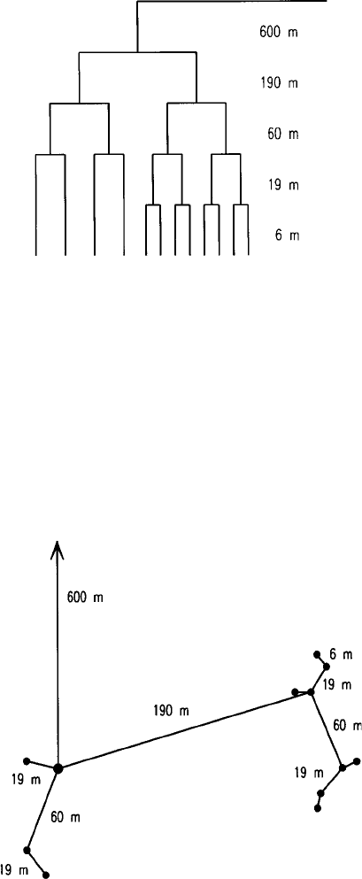
From each grid node a second site was chosen 190 m away to provide the

second stage. From each of the now 18 sites another point was chosen 60 m

away (stage 3). The procedure was repeated at stage 4 to locate points 19 m

away from those of stage 3, giving 72 points. At the ﬁfth stage just half of the

fourth-stage points were replicated by sampling 6 m away. This gave a

sample of 108 points rather than 144 for a fully balanced survey. Table 6.7

summarizes the design, Figure 6.13 illustrates the hierarchical structure used

for one centre, and Figure 6.14 shows the conﬁguration of sampling points for

Figure 6.13 Topology for one main centre of the unbalanced nested sampling as

implemented in the soil survey of the Wyre Forest by Oliver and Webster (1987).

Figure 6.14 Sampling plan for one main centre of the Wyre Forest survey (not strictly

to scale).

Theory of Nested Sampling and Analysis 135

one ﬁrst-stage centre. The design achieved a 25% economy in effort compared

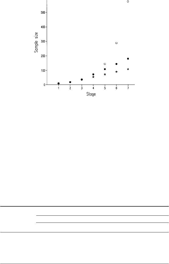
with a fully balanced scheme. Figure 6.15 shows the economy possible

with even more stages. At each sampling point seve ral properties of the soil

were recorded at four ﬁxed depths in the soil proﬁle: 0–5 cm (1), 10–15 cm (2),

25–30 cm (3), and 50–55 cm (4).

Each variable was analysed by ANOVA according to the scheme outlined in

Table 6.8 and by REML with and without the components’ bein g constrained to

be non-negative. The estimated components of variance for sand content at the

four depths are listed in Table 6.8 for ANOVA. Figure 6.16(a) shows the

accumulated components of variance for each dept h in the proﬁle plotted

Figure 6.15 Graph showing the economy achieved by not doubling the sampling at

every level in the hierarchy. The symbols are  balanced design,  Wyre Forest scheme

including extension to stages 6 and 7, ? scheme used by Webster and Boag (1992) in

their surveys of nematode infestations.

Table 6.8 Components of variance of sand content of the soil at four depths in the

survey of the Wyre Forest estimated by analysis of variance.

Component of variance

Depth/cm

Stage 0–5 10–15 25–30 50–55

1 (600 m) 32.44 17.54 27.95 32.63

2 (190 m) 51:90 64:82 81:97 103:44

3 (60 m) 88.77 141.79 172.02 316.28

4 (19 m) 139.44 101.10 135.21 45.79

5 (6 m) 55.58 68.42 116.33 309.73

136 Reliability of the Experimental Variogram and Nested Sampling