Webster R., Oliver M.A., Geostatistics for Environmental Scientists

Подождите немного. Документ загружается.

kriging



gðB; BÞ becomes gðx

; x

Þ¼0, which is why equation (8.2) has two

terms rather than three.

For each kriged estimate there is an associated kriging variance, which we

can denote by s

ðx

Þ and s

ðBÞ for the point and block, respectively, and which

are deﬁned in equations (8.2) and (8.4). The next step in kriging is to ﬁnd the

weights that minimize these variances, subject to the constraint that they sum

to 1. We achieve this using the method of Lagrange multipliers.

We deﬁne an auxiliary function f ðl

; cÞ tha t contains the variance we wish

to minimize plus a term containing a Lagrange multiplier, c. For punctual

kriging it is

Tðl

; cÞ¼var½

Zðx

Þzðx

Þ  2c

i¼1

 1

()

: ð8:7Þ

We then set the partial derivatives of the function with respect to the weights

to 0:

@f ðl

; cÞ

¼ 0;

@f ðl

; cÞ

¼ 0; ð8:8Þ

for i ¼ 1; 2; ...; N. This leads to a set of N þ 1 equations in N þ 1 unknowns:

i¼1

gðx

; x

Þþcðx

Þ¼gðx

; x

Þ for all j;

i¼1

¼ 1: ð8:9Þ

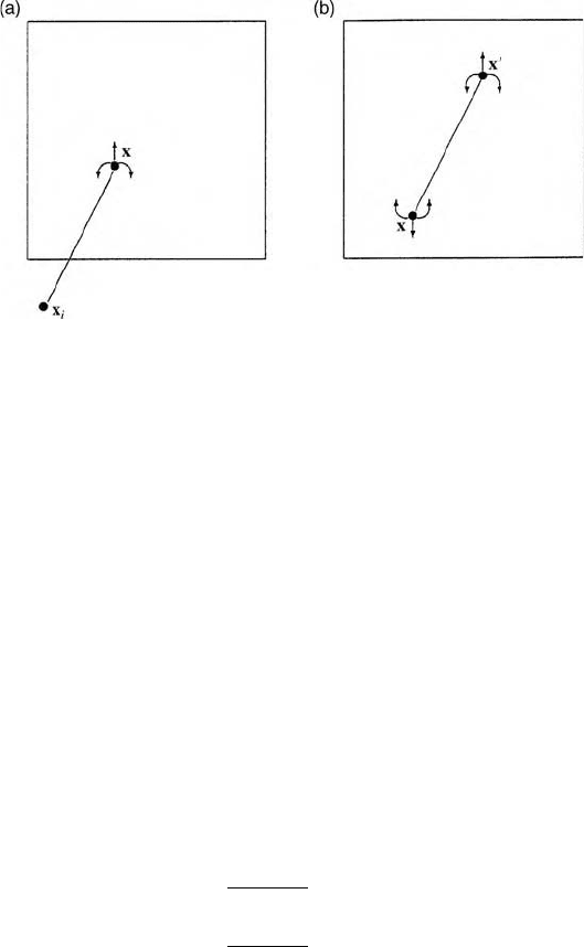
Figure 8.1 Integration of the variogram: (a) between a sampling point and a block; (b)

within a block.

Theory of Ordinary Kriging 157

This is the ordinary kriging system for points. Its solution provides the weights, l

which are entered into equation (8.1), and from which the estimation variance

(prediction variance or speciﬁcally kriging variance) can be obtained as

ðx

Þ¼

i¼1

gðx

; x

Þþcðx

Þ: ð8:10Þ

If a target point, x

, happens to be one of the data points, say x

, then s

ðx

Þ is

minimized when lðx

Þ¼1 and all of the other weights are 0. In fact, s

ðx

Þ¼0,

and by inserting the weights into equation (8.1) we obtain the recorded value,

zðx

Þ, as our estimate of zðx

Þ. Punctual kriging is thus an exact interpolator.

The equivalent kriging system for blocks is

i¼1

gðx

; x

ÞþcðBÞ¼



gðx

; BÞ for all j;

i¼1

¼ 1; ð8:11Þ

with the associated variance obtained as

ðBÞ¼

i¼1



gðx

; BÞþcð BÞ



gðB; BÞ: ð8:12Þ

The kriging equations can be represented in matrix form. For punctual

kriging they are

Al ¼ b ð8:13Þ

where

A ¼

gðx

; x

Þ gðx

; x

Þ  gðx

; x

Þ 1

gðx

; x

Þ gðx

; x

Þ  gðx

; x

Þ 1



gðx

; x

Þ gðx

; x

Þ  gðx

; x

Þ 1

11 10

;

l ¼

cðx

and b ¼

gðx

; x

gðx

; x

gðx

; x

158 Local Estimation or Prediction: Kriging

Matrix A is inverted, and the weights and the Lagrange multiplier are obtained

l ¼ A

1

b: ð8:14Þ

The krig ing variance is given by

ðx

Þ¼b

l: ð8:15Þ

For block kriging the only differences are that

b ¼



gðx

; BÞ



gðx

; BÞ



gðx

; BÞ

and

ðBÞ¼b

l 



gðB; BÞ: ð8:16Þ

8.3 WEIGHTS

When the kriging equations are solved to obtain the weights, l

, in general the

only large weights are those of the points near to the point or block to be kriged.

The nearest four or ﬁve might contribute 80% of the total weight, and the next

nearest ten almost all of the remainder. The weights also depend on the

conﬁguration of the sampling. We can summarize the factors affecting the

weights as follows.

1. Near points carry more weight than more distant ones. Their relative

proportions depend on the positions of the sampling points and on the

variogram: the larger is the nugget variance, the smaller are the weights of

the points that are nearest to target point or block.

2. The relative weights of points also depend on the block size: as the block size

increases, the weights of the nearest points decrease and those of the more

distant points increase (Figure 8.9), until the weights become nearly equal.

3. Clustered points carry less weight individually than isolated ones at the

same distance (Fig ure 8.12).

Weights 159

4. Data points can be screened by ones lying between them and the target

(Figure 8.12).

These effects are all intuitively desirable, and the ﬁrst shows that kriging is local.

They will become evident in the examples below. They also have practical

implications. The most important for present purposes is that because only the

nearest few data points to the target carry signiﬁcant weight, matrix A in the

kriging system need never be large and its inversion will be swift. We can

replace N in equations (8.9) and (8.11) by some much smaller number, say

n  N. We shall reiterate this below after the examples in which we set n to 16.

8.4 EXAMPLES

This section shows the effects of a changing variogram, target point and

sampling intensity on the weights in a way analogous to the kriging exercises

in GSLIB (Deutsch and Journel, 1992). It uses the data on pH from Broom’s

Barn Farm for the purpose. We have chosen pH because it is easy to appreciate

changes in the estimated values and because we can start with a simple

isotropic exponential model without nugget (Figure 8.2), which is the best-

ﬁtting model:

gðhÞ¼cf1  expðh=r Þg; ð8:17Þ

with c ¼ 0:382 and r ¼ 90:53 m, i.e. an effective range ða

¼ 3rÞ of approxi-

mately 272 m (Table 8.1). We have also selected n ¼ 16 points on a 4  4 lattice

from the full set of data (Figure 8.3). There are also three separate target points,

one at the centre of the lattice, Figure 8.3(a), one off-centre, Figure 8.3(b), and a

0.5

0.4

0.3

0.2

0.1

Variance

0 100 200 300 400

Lag distance/m

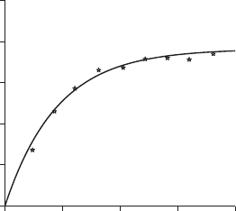
Figure 8.2 Variogram of pH at Broom’s Barn Farm. The points are the experimental

semivariances, and the solid line is the best ﬁtting exponential model, the parameters of

which are given in the text.

160 Local Estimation or Prediction: Kriging

third coinciding with one of the sampling points, Figure 8.11(c). Using equation

(8.9) and the 16 points we estimated the values at the target points as follows.

8.4.1 Kriging at the centre of the lattice

Changing the ratio of nugget:sill variance

Figure 8.4(a) shows the weights derived using the best-ﬁtting model to pH

(exponential N1, Table 8.1; and exponential R2, Table 8.2). The weights of the

four points nearest to the target point are large and positive, and their sum

exceeds 1. To ensure unbiasedness the sum of all the weig hts must be 1, and

hence the weights of the outer points are negative. In this case the outer points

are close to 0 and so have little inﬂuence on the esti mate.

We now change the variogram by introducin g a nugget variance, c

¼ 0:1

(the model para meters are those of exponential N2 in Table 8.1). The resulting

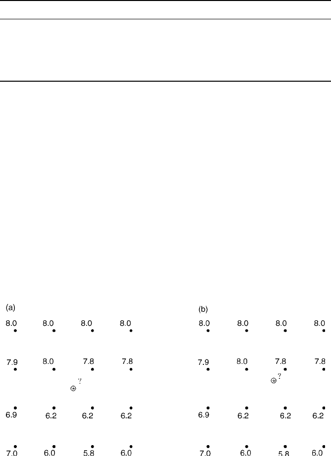
Figure 8.3 The grid of 16 sample values selected from Broom’s Barn Farm with the pH

values given for each sampling location. The point to be estimated is located: (a)

centrally; (b) off-centre.

Table 8.1 Model parameters with changing ratio of nugget:sill variance and ﬁxed

distance parameter, r ¼ 90:53 m, equivalent to an effective range of 271.6 m.

Model c

Exponential N1 0 0.3820

Exponential N2 0.1 0.2820

Exponential N3 0.3 0.0820

Exponential N4 0.382 0

(Pure nugget) 1 0

Examples 161

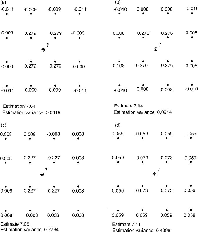
Figure 8.4 Kriging weights from punctual kriging of pH with an exponential function

with the distance parameter r ¼ 90:53 m, and changing the nugget:sill variance:

(a) c

¼ 0, c ¼ 0:382; (b) c

¼ 0:1, c ¼ 0:282; (c) c

¼ 0:3, c ¼ 0:082; (d) c

0:382, c ¼ 0.

Table 8.2 Model parameters with changing distance parameter, r, for exponential

model.

Model c

cr/m Effective range/m

Exponential R1 0 0.382 133.3 400.00

Exponential R2 0 0.382 90.53 271.59

Exponential R3 0 0.382 26.67 80.00

Exponential R4 0 0.382 6.67 20.00

162 Local Estimation or Prediction: Kriging

weights are shown in Figure 8.4(b): those of the inner four points have

decreased somewhat, whilst those of the outer points have increased and are

now all positive. The weights of the corner points of the lattice are the smallest

because they are the furthest from x

Figure 8.4(c) shows the weights obtained by increasing the proportion of

nugget more substantially so that it dominates (the model parameters are those of

exponential N3 in Table 8.1). The weights of the inner points have decreased

considerably, and those of the outer ones have increased correspondingly.

For a pure nugget variogram, with parameters exponential (N4) in Table 8.1,

the weights are all the same (Figure 8.4(d)). The result is the same as if we had

sampled at random in classical estimation; the kriging variance is the variance

of the process, c

, plus the variance of the mean, given by cðx

). The solution of

equation (8.15) is

þ cðx

Þ¼0:382 þ 0:0625 ¼ 0:4445: ð8:18Þ

Figure 8.5(a) summarizes the shapes of the exponential variogram models

that resulted from changing the ratio of nugget:sill variance and keeping the

distance parameter constant.

The estimated value for pH and kriging variance are given for each of the

above examples (Figure 8.4). The estimated value changes each tim e: we can

assume that 7.04 is the optimal estimate because it was derived from the

best-ﬁtting model. The average pH of the 16 values is 7.11, which is also the

estimate returned with a pure nugget variogram and for which the kriging

variance is the largest. The kriging variance increases as the nugget variance

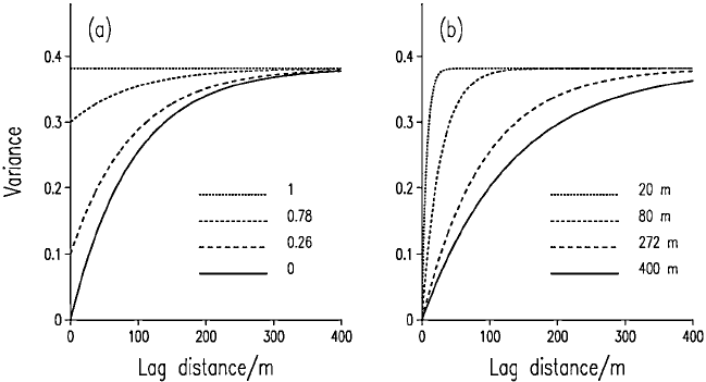
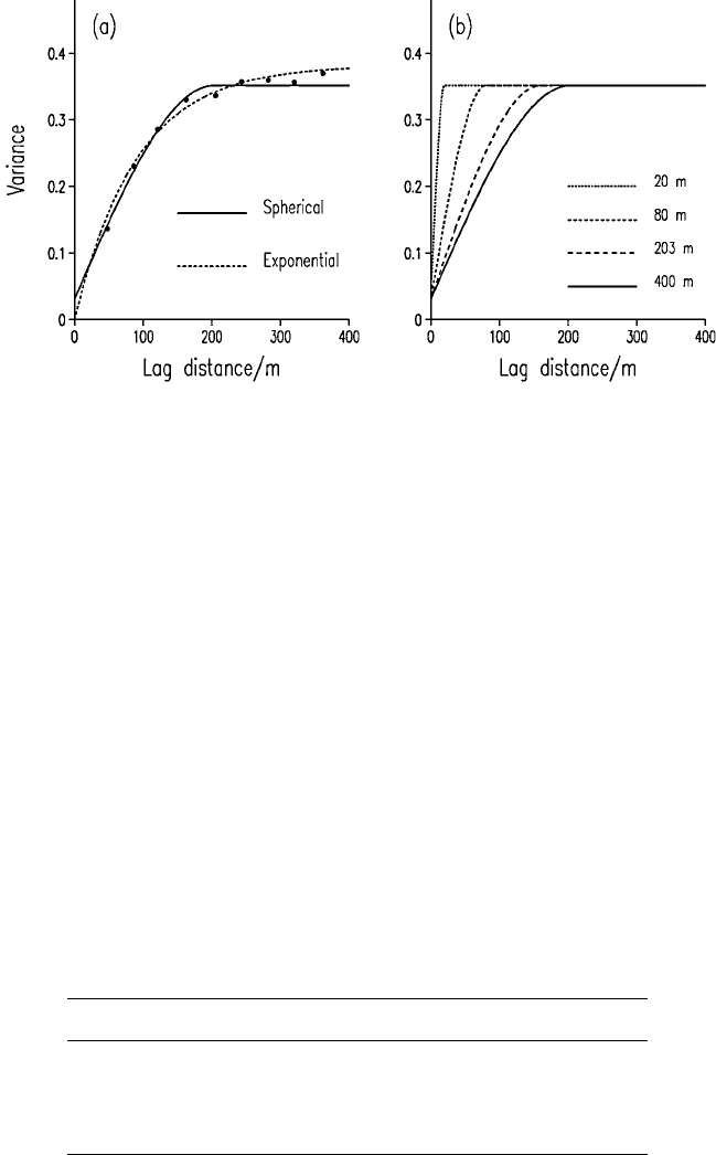
Figure 8.5 (a) Exponential variograms used to obtain the weights in Figure 8.4 with

the distance parameter r ¼ 90:53 m, and changing the nugget:sill variance: 0:0.382;

0.1:0.282; 0.3:0.082; 0.382:0. (b) Effect on the exponential variogram of changing the

effective range (a

¼ 3r) with c

¼ 0 and c ¼ 0:382: a

¼ 400, 271.59, 80, 20.

Examples 163

increases, as we sho uld expect, because the grea ter the variance that remains

unresolved the more uncert ain is the estimate. The estimates and their

associated variances illustrate two points:

(i) A nugget variance increases the kriging variance, and for punctual kriging

it sets a lower limit to that variance (see Figures 8.17 and 11.8(b)).

(ii) It is important to ﬁt the model correctly to the sample semivariances

because of the effect of the model on both the estimates and their variances.

Although the kriging variances are smaller for a smaller nugget variance, the

model must represent the nugget effect realistically. If it does not then the

estimates could be judged to be more or less reliable than they really are.

Changing the range or sampling intens ity

We now explore the effect of decreasing the range of spatial dependence, or, what

amounts to the same thing, decreasing the sampling density. The nugget variance

and the sill of the spatially dependent component, c, were kept constant and we

changed the distance parameter, as shown in Table 8.2. Figure 8.5(b) shows the

effect on the shape of the exponential variogram, and Figure 8.6(a) shows the

weights for exponential R1, where the effective range of dependence (a

¼ 3r)is

400 m. The weights of the inner four points are the largest, and the outer ones

contribute little or nothing. If we compare this with Figure 8.6(b) for the best-

ﬁtting exponential model R2, it is clear that they are similar. As the effective range

lengthens, however, the inner points gain weight in accordance with the increase

in spatial continuity in the variation. If we reduce the effective range substantially

to 80 m (exponential (R3)), then the weights of the inner points decrease and

those of the outer ones increase (Figure 8.6(c)). When we reduce the effective

range to half the sampling interval, i.e. 20 m (exponential R4), the variogram is

effectively pure nugget. Figure 8.6(d) shows the weights which are now small for

all of the points, though they are not all the same: the inner ones are somewhat

larger than the outer ones, because with the exponential model the distance

parameter does not disappear completely. Nevertheless, the estimate is the mean

of the data as in the previous example, Figure 8.4(a), but the kriging variance is a

little less because of the effect of the differences in the weights.

Since changing the distance parameter of a spherical model has a different

effect, we include the results of changing the range of the best-ﬁtting spherical

function to the 16 points. The spherical function is give n by

gðhÞ¼c

þ c





()

; ð8:19Þ

with the parameter values c

¼ 0:0309; c ¼ 0:3211 and a ¼ 203:2 m for the

best-ﬁtting spherical function.

164 Local Estimation or Prediction: Kriging

There are several interesting differences between the results of these models.

Figure 8.7(a) shows the best-ﬁtting spherical and exponential models ﬁtted to

pH, and Figure 8.7(b) shows the effect of changing the range on the shape of

the spherical model.

To compare the weights with those for the exponential model we started with

spherical A1 of Table 8.3, with a range of 400 m. The weights of the inner

Figure 8.6 Kriging weights from punctual kriging of pH with an exponential function

with c

¼ 0 and c ¼ 0:382, and changing the effective range (a

¼ 3r): (a) a

¼ 400; (b)

¼ 203:2; (c) a

¼ 80:0; (d) a

¼ 20:0.

Examples 165

points are smaller, and those of the outer ones larger, than those for the

exponential model, Figure 8.8(a). This is because the spheric al model has a

small nugget variance, whereas the exponential had none, and there is a

difference in the curvature of these two models (Figure 8.7(a)). Figure 8.8(b)

shows the weights obtained when using the best-ﬁtting spherical function,

spherical A2; the inner weights are larger and the outer ones slightly smaller. It

is a reversal of the effect with the exponential model. When the range is reduced

to 80 m, spherical (A3), the inner weights, Figure 8.8(c), are much larger than

for the equivalent exponential model, Figure 8.6(c), again because of the effect

of the model’s curvature. Finally, when the range is 20 m the weights are all the

same, Figure 8.8(d), and the observed effect is the same as that for the pure

nugget variogram. In this situation all of the variatio n occurs within the

sampling interval. It illustrates clearly that if the distance over which most of

the variation occurs is less than the sampling interval then the simple formula for

random sampling gives the best estimate for an unsampled point, which is the

mean of the data. It also shows the importance of sampling sufﬁciently densely to

estimate the variogram at the spatial scale of the investigation.

Figure 8.7 (a) The best-ﬁtting spherical (solid line) and exponential (dashed line) ﬁtted

to the experimental variogram of pH. (b) Spherical variograms used to obtain the weights

in Figure 8.8 with c

¼ 0:031, c ¼ 0:321, and range a ¼ 203: 2 m, 160 m, 80 m, 20 m.

Table 8.3 Parameters with the range changing for spherical model.

Model c

c Range/m

Spherical A1 0.0309 0.3211 400.0

Spherical A2 0.0309 0.3211 203.2

Spherical A3 0.0309 0.3211 80.0

Spherical A4 0.0309 0.3211 20.0

166 Local Estimation or Prediction: Kriging