Webster R., Oliver M.A., Geostatistics for Environmental Scientists

Подождите немного. Документ загружается.

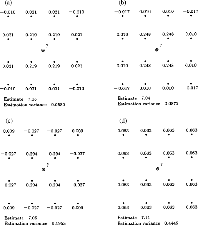
In summary, Figure 8.8(a)–(c) shows that as the distance parameter

decreases the weights of the inner points increase and those of the outer ones

decrease. Apart from Figure 8.8(a), the estimates are sensibly the same as those

for the exponential model, but the kriging variances for the spherical mod el are

smaller in every case.

Figure 8.8 Kriging weights from punctual kriging of pH with a spherical function with

¼ 0:031, c ¼ 0:321, and changing the distance parameter (range): (a) a ¼ 400 m;

(b) a ¼ 203:2 m; (c) a ¼ 80 m; (d) a ¼ 20 m.

Examples 167

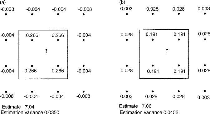
Kriging over a block

The results for block kriging over a centrally located 80 m  80 m block with

the parameters of the best-ﬁtting exponential model (N1 in Table 8.1), are

shown in Figure 8.9(a), and those with exponential (N2) in Figure 8.9(b). A

comparison of the weig hts in Figures 8.4(a) and 8.9(a) shows that by increas-

ing the bloc k size the inner weights decrease and the outer ones increase. The

differences between the two ﬁgures are small, but the kriging variance for block

kriging with this model is only a little more than a third of that for punctual

kriging. With a modest nugget variance, exponential N2, the relative decrease

in the inner weights for block kriging, Figure 8.9(b), is somewhat less than in

Figure 8.4(b), but the decreas e in the kriging variance over that of punctual

kriging is even more marked; it is now less than a quarter. Nevertheless, the

estimated values are the same in each case.

This comparison shows two effects of the nugget variance as foll ows:

1. The nugget variance sets a lower limit to the punctual kriging variance.

2. The nugget variance disappears from the block-krigin g variance; see

equations (8.4) and (8.12). Therefore, the larger is the proportion of

the nugget variance, which is taken out of consideration, the smaller

is the block-kriging variance and the greater is the difference between it and

the pun ctual kriging variance.

It also raises an important issue of conﬁdence. When practitioners ﬁt models to

variograms, whether by eye or by minimizing some function of the residuals, they

Figure 8.9 Kriging weights from block kriging of pH over a centrally located block of

80 m  80 m: (a) for the best-ﬁtting exponential model with c

¼ 0, c ¼ 0:382 and

r ¼ 90:53 m; (b) with c

¼ 0:1, c ¼ 0:282 and r ¼ 90:53 m.

168 Local Estimation or Prediction: Kriging

project their models towards the ordinate with the least change in curvature. They

know nothing about the shape of the variogram at distances less than the shortest

lag interval, and the practice may be regarded as prudent. The intercept gives them

a nugget variance that is almost certainly larger than any error of measurement or

short-range spatial component. When the model is used for punctual kriging the

errors will, therefore, tend to be on the large side; the estimates are conservative.

However, when the same model is used for block kriging, if the nugget variance is

exaggerated then the kriging variance will be too small for the reasons given

above, and the practitioner will obtain a false sense of conﬁdence.

The effect of anisotropy

We examine the effect of geometric anisotropy on the weights by punctual

kriging with the exponential model

gðh;#Þ¼cf1  expðh=VÞg; ð8:20Þ

where

V ¼

ﬃﬃﬃﬃﬃﬃﬃﬃﬃﬃﬃﬃﬃﬃﬃﬃﬃﬃﬃﬃﬃﬃﬃﬃﬃﬃﬃﬃﬃﬃﬃﬃﬃﬃﬃﬃﬃﬃﬃﬃﬃﬃﬃﬃﬃﬃﬃﬃﬃﬃﬃﬃﬃﬃﬃﬃﬃﬃﬃﬃﬃﬃﬃﬃﬃ

cos

ð#  ’ÞþB

sin

ð#  ’Þ

; ð8:21Þ

in which A ¼ 271:6; B ¼ 90:5 and ’ ¼ p=2 ¼ 0:7854 rad or 45



. The angle

’ is the direction of maximum continuity, i.e. largest effective range, as in

Figure 5.13. The ratio A=B is the anisotropy ratio, and is 3 ¼ 271:6=90:5.

Figure 8.10(a) shows the weights for the isotropic variogram and Figure 8.10(b)

those for the anisotropic function. The largest weights are at the points adjacent

to the target point along the 45



diagonal.

There is a marked decrease in the weights of the adjacent points at right

angles. The changes in the weights of the outer points are far less marked.

If we change ’ to 0.2618 rad, or 15



(75



in geographical notation) then

Figure 8.10(c) ensues; the distribution of the weights has changed. The increase

in the weights of the nearest points is less dramatic, but the outer weights close

to the (15



) line have increased substantially to 0.153.

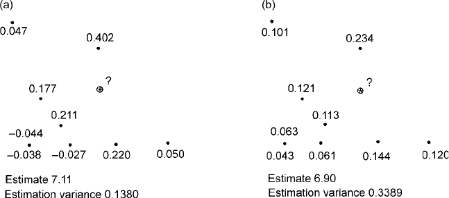
8.4.2 Kriging off-centre in the lattice and at a sampling point

Let us now use the exponential models (Table 8.1), one with no nugget N1 and

the other with a nugget variance of 0.1 N2, to estimate the valu e at a target

point that is off-centre but on a diagonal of the grid (Figure 8.11). In both

Figure 8.11(a) and 8.11(b) the point closest to the target has the largest weight,

and the point diagonally opposite has the smalles t weight of the four inner

points. The other two inner points have the same weights because they are

equidistant from the target. The weig hts of the outer points now show the effect

Examples 169

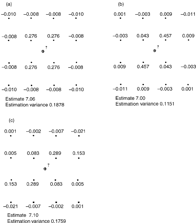
of screening. Figure 8.11(a) shows that the unscreened outer points have

positive weights, whereas those that are screened are negative.

The weights in Figure 8.11(c) were obtained by solution of the kriging system

for punctual kriging at the target point coinciding with the sampling location

indicated. They are 1 at the sampling point and 0 elsewhere, which is what we

should expect from theory. The estimate is the sample value, and the estimation

variance is 0, so illustrating that ordinary punctual kriging is an exact

interpolator. The weights in Figure 8.11(d) were obtained with the sam e model

Figure 8.10 Kriging weights from punctual kriging of pH: (a) for the best-ﬁtting

exponential model with c

¼ 0, c ¼ 0:382, and r ¼ 90:53 m; (b) for an anisotropic

exponential model with the direction of maximum variation p=2 radians and an

anisotropy ratio of 3; (c) with the direction of maximum variation 1.309 rad.

170 Local Estimation or Prediction: Kriging

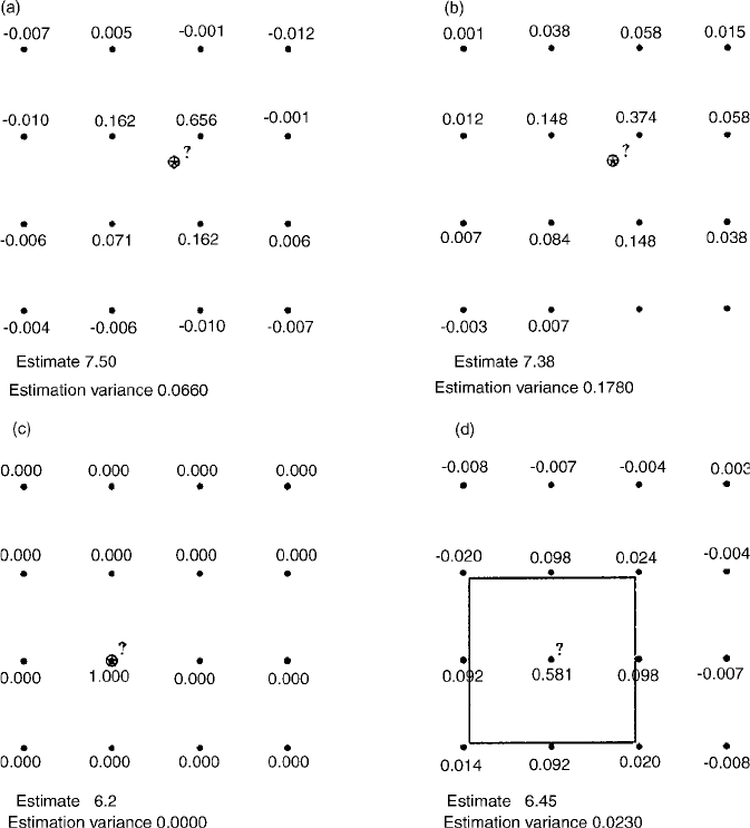
and kriging over a 80 m  80 m block centred at the same sampling point. The

weight at the sampling location is an order of magnitude larger than tho se of

the surroundi ng nearest points, while those of the outer edges are negative. The

estimate is substantially different from the measured value at the centre of the

Figure 8.11 Kriging weights of pH with the exponential function: punctual kriging

with the point to be estimated off-centre and the model: (a) c

¼ 0, c ¼ 0:382,

r ¼ 90:53 m; (b) c

¼ 0:1, c ¼ 0:282, r ¼ 90:53 m; (c) with the point to be estimated

at a sampling location with c

¼ 0, c ¼ 0:382, r ¼ 90:53 m; (d) block kriging with an

80 m  80 m block centred at a sampling point with c

¼ 0, c ¼ 0:382 and r ¼ 90:53 m.

Examples 171

block and shows the smoothing effect of block kriging. The kriging variance is

also very small, but not zero.

8.4.3 Kriging from irregularly spaced data

Figure 8.12 shows an irregular conﬁguration of nine sampling points plus a

target point; the nine are a sele ction from the 16 values used previously, but

some of the locations were changed. The weig hts in Figure 8.12(a) were

obtained with the best-ﬁtting exponential model N1, and punctual krig ing.

Those in Figure 8.12(b) were derived with exponential N2. The two diagrams

show more clearly than those for the grid the effect of the data conﬁguration on

the weights. Points that are clustered carry less weight relative to isolated ones.

The point to the north of the target carries almost twice the weight of the next

most important point because it is far from any other point. The poin ts that are

screened by others have negative weights.

8.5 NEIGHBOURHOOD

The notion of the neighbourhood embodies the local nature of kriging, and it

confers advantages on the method, as follows.

1. Only the nearest few points to the target point or block carry signiﬁcant

weight, therefore the kriging system need never be large and inverting

matrix A will be swift. We can replace N in equations (8.9) and (8.11) by a

much smaller n  N. This might not matter when krig ing only one point

or block, but for mapping in which many estimates are needed it can make

a big difference because the time required to invert a matrix is approxi-

Figure 8.12 Kriging weights from punctual kriging of pH with an exponential model

and irregularly scattered sampling points: (a) c

¼ 0, c ¼ 0:382 and r ¼ 90:53 m;

(b) c

¼ 0:2, c ¼ 0:182 and r ¼ 90:53 m.

172 Local Estimation or Prediction: Kriging

mately proportional to the cube of its order. It also avoids instability that

can arise with large matrices.

2. If only the points near to the target carry signiﬁcant weight then the

variogram need be estimated and modelled well only at short lag distances,

and in fact this is usually where the variogram is best estimated. The

widening of the conﬁdence intervals on the expe rimental variogram is

somewhat less serious than it might appear from Chapter 5. This adds to

the desirability of giving most weight to the experimental semivariances at

the short lags when modelling the variogram.

3. The local nat ure of ordinary kriging means that what happens over large

distances is of little consequence for the estimates. We can accept the notion

of quasi-stationarity, i.e. local stationarity (Chapt er 4), compute the

variogram over only short distances, and apply it without taking account

of long-range ﬂuctuations in E½ZðxÞ. The assumptions underpinning the

method are not violated. It is perhaps this feature that has made ordinary

kriging the ‘workhorse’ of geostatistics.

There are no strict rules for deﬁning the neighbourhood, but we suggest some

guidelines as follows:

1. If the variogram is bounded and has a small nugget variance and the data are

dense then the radius of the neighbourhood can be set close to the range or

effective range. Any data beyond the range will have negligible weights.

2. If data are sparse, however, points beyond the ran ge from the target might

carry sufﬁcient weight to be important, and the nei ghbourhood should be

such as to include them.

3. If the nugget variance is large, then again distant points are likely to carry

signiﬁcant weight.

4. As an alternative, the user may choose the nearest n data points, and

effectively let this number limit the neighbourhood. If the sampling con-

ﬁguration is irregular then the size of the neighbourhood will vary more or

less as the target point is moved. We have found that a maximum of n  20

is usually enough.

5. If you set a maximum radius for the neighbourhood then you may also

need to set a minimum for n, especially to cater for targets near the

boundary of a region. A value of n  7 is likely to be satisfactory.

6. Where the scatter is very uneven good practice is to divide the space around

the target point into octa nts and take the nearest two points in each.

Several kriging programs do this as a matter of course.

We recommend that when you start to analyse new data you examine what

happens to the kriging weights as you change the neighbourhood. This is especi-

ally important in mapping where you move the neighbourhood. In these circum-

stances the most distant points should have zero weight so that the estimated

surface appears seamless; see Laslett et al. (1987) for an illustrated discussion.

Neighbourhood 173

8.6 ORDINARY KRIGING FOR MAPPING

Kriging was developed in mining originally to estimate the amounts of metal in

blocks of rock, and it is still used in this way. In these circumstances every block

of rock is potentially of interest, and its metal conten t will be estimated. The

miner may then deci de whether the rock contains sufﬁcient metal to be mined

and sent for processing. Environmental scientists, and pedologists in particular,

have used kriging in a rather different way, namely optimal interpolation at

many places for mapping. The earliest examples are those by Burges s and

Webster (1980a, 1980b) and Burgess et al. (1981), who used ordinary kriging.

There have been many since, for example Mulla (1997), Frogbrook (1999) and

Frogbrook et al. (1999) in precision agriculture.

To map a variable the values are kriged at the nodes of a ﬁne grid. Isarithms

are then threaded through this grid, and there are now many programs and

packages, such as Surfer (Golden Software, 2002) and Gsharp, and geographi-

cal information systems, such as Arc/Info, that will do this with excellent

graphics. Computing the isarithms involves another interpolation which is

rarely optimal in the kriging sense, but if the kriged grid is ﬁne enough this lack

of optimality is immaterial. In most instances kriging at intervals of 2 mm on

the ﬁnished map will be adequate.

The kriging variances and their square roots, the kriging errors, can be

mapped similarly, and these maps give an idea of the reliability of the maps of

estimates.

Creating a grid of kriged values to make a map can involve heavy computa-

tion. In principle all the estimates and the ir variances could be fou nd from a

single inversion of matrix A in equation (8.13) that contains all of the

semivariances between the sampling sites. As above, however, this is unwise

or even impossible when the matrices are large. In practice, therefore, one

enters into A only the semivariances for some n data points, i.e. within the

neighbourhood, near each grid node. This keeps the matrix small, but increases

the number of inversions needed. Inversion can be accelerated if you work with

the covariances instead of the semivariances because in the usual method of

matrix inversion the largest element in each row, which serves as a pivot, is

always in the diagonal of the covariance matrix and need not be sought.

For variables that are second-order stationary all the formulae for ﬁnding the

weights from the variogram also apply to the covariance function with only

changes of sign. For variables that are intrinsic only, the technique can still be

used if you take some arbitrary large value for the covariance at h ¼ 0.

Other economies can be made depending on the location of the sampling

points. If they are irregularly scattered then the same few data will often be used

to estimate ZðxÞ at several grid nodes within a small area. Furthermore, the

ﬁner the interpolation grid the more nodes can be interpolated from the same

observations. Matrix A remains the same and needs inverting only once. Much

174 Local Estimation or Prediction: Kriging

larger economies are possible where the data are on a regular grid because the

same conﬁguration recurs many times. Not only does the variogram remain

constant, but so also does matrix A for any given conﬁguration. Each conﬁg-

uration requires only one matrix inversion. If sampling has been done on a

square grid and the interpolation grid ﬁts on to it with interval 1=r times that of

the sampling grid then there are only r

possible conﬁgurations except near to

the edge of the map. Where variation is isotropic the spatial relations have a

fourfold symmetry, so even fewer solutions are needed.

8.7 CASE STUDY

To illustrate the application of kriging to mapping we return to the analysis of

exchangeable potassium (K) from Broom’s Barn Farm. Since the distribution of

K is skewed (skewness 2.04, Table 2.1) we transformed the values to common

logarithms (log

K) which reduced the skewness to 0.39.

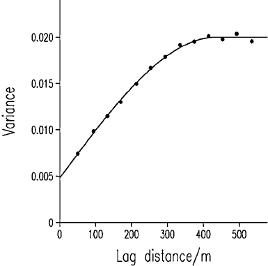
The variogram was computed on the transformed data, and the experimental

semivariances were ﬁtted best by a spherical function, equation (8.19), by

weighted least-squares approximation as described in Chapter 5. The resulting

coefﬁcients are c

¼ 0:0048; c ¼ 0:015 19 and a ¼ 439:2 m. Figure 8.13

shows the experimental variogram (symbols) and the ﬁtted spherical model

(solid line). This function was then used for the kriging. We set the maximum

radius of the neighbourhood to 400 m, and we set the minimum number of

Figure 8.13 Variogram of exchangeable potassium at Broom’s Barn Farm trans-

formed to common logarithms. The points are the experimental semivariances, and the

solid line is the best-ﬁtting spherical model, the parameters of which are given in the text.

Case Study 175

points to seven and the maximum to 20. We kriged at intervals of 10 m, and for

the block kriging our blocks were 50 m  50 m. The estimated values and

kriging variances hav e been mapped with Gsharp.

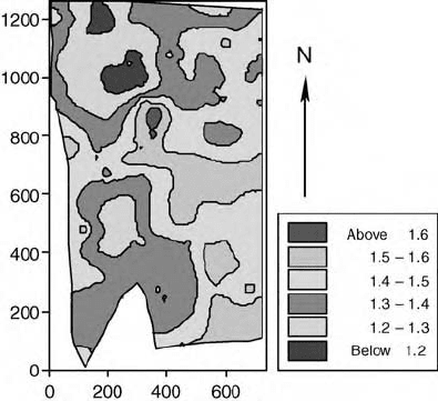
Figure 8.14 is a map of the punctual estimates. For it we deliberately placed

the kriging grid over the sampling grid so that the sampling points lay on it to

illustrate the nugget effect. The map is somewhat ‘spotty’ because we have

kriged at the data points. The spatial pattern of log

K is distinctly patchy, as we

should expect from the spherical variogram; there are patches of large values

and patc hes of small ones. The average extent of the patches is about 400 m.

In the alternative representation as a perspective diagram (Figure 8.15), the

spots now appear as spectacular spikes, both above and below the surface. The

reason is that at the sampling points punctual kriging returns the measured

values there, whereas elsewhere it forms weighted averages of the data. The

nugget variance in the variogram represents a discontinuity (Chapter 5), and

this continues through to the kriging. Another way of viewing the effect is to

consider the esti mate as comprising two parts: the nugget variance and the

continuous autocorrelated variation. Combining these two components pro-

duces the effect. The larger is the nugget variance as a proportion of the total

variance the more pronounced this effect becomes; when all of the variance is

nugget the surface becomes ﬂat between the sampling points.

Figure 8.16 is a map of the block estimates which has lost the ‘spotty’

appearance of Figure 8.14. Nevertheless, the same broad pattern in the

distribution of log

K is evident. The block-kriged surface is smoother, and

this is evident in the perspective diagram of this surface, shown in Figure 8.17.

Figure 8.14 Map of exchangeable potassium, transformed to common logarithms, at

Broom’s Barn Farm made by punctual kriging on a 10 m  10 m grid that coincided

with the sampling grid. The units are log

(mg K l

1

Þ.

176 Local Estimation or Prediction: Kriging