Webster R., Oliver M.A., Geostatistics for Environmental Scientists

Подождите немного. Документ загружается.

Matheron elaborated the ordinary kriging system to take into account the ﬁxed

effects of the trend in addition to the random component as

i¼1

gðx

; x

Þþc

k¼0

ðx

Þ¼gðx

; x

Þ for all j ¼ 1; 2: ...; N;

i¼1

¼ 1; ð9:10Þ

i¼1

ðx

Þ¼ f

ðx

Þ for all k ¼ 0; 1; ...; K:

The values gðx

; x

Þ are the semivariances of the residuals between the data

points x

and x

,andthegðx

; x

Þ are the semivariances between the target point

and the data points. The functions f

ðxÞ refer to an origin x ¼ 0 for the target

point x

. For a linear drift there are three functions, i.e. K þ 1 ¼ 3, with values

¼ 1; f

¼ x

; f

¼ x

For quadratic drift there are three additional functions:

¼ x

; f

¼ x

; f

¼ x

In addition there are now three Lagrange multipliers, c

; c

and c

, for the

linear drift and three more, c

; c

and c

, for quadratic drift.

The universal kriging system, like that for ordinary kriging, is a set of linear

equations which we can represent in matrix notation by

Al ¼ b; ð9:11Þ

as in equation (8.13). Now, however, the matrix A and the vectors l and b are aug-

mented with functions of the spatial positions of the data points and of the target:

A ¼

gðx

; x

Þ gðx

; x

Þgðx

; x

Þ 1 f

ðx

Þ f

ðx

Þf

ðx

gðx

; x

Þ gðx

; x

Þgðx

; x

Þ 1 f

ðx

Þ f

ðx

Þf

ðx



gðx

; x

Þ gðx

; x

Þgðx

; x

Þ 1 f

ðx

Þ f

ðx

Þf

ðx

11 100 0 0

ðxÞ

ðx

Þf

ðx

Þ 00 0 0

ðxÞ

ðx

Þf

ðx

Þ 00 0 0



ðxÞ

ðx

Þf

ðx

Þ 00 0 0

;

Non-Stationarity in the Mean 197

l ¼

and b ¼

gðx

; x

gðx

; x

gðx

; x

ðx

As in ordinary kriging, A is inverted, and the weights and the Lagrange

multipliers are obtained as

l ¼ A

1

b: ð9:12Þ

The weights are inserted into equation (9.7), and the kriging variance is given

¼ b

l: ð9:13Þ

Also as in ordinary kriging, we can usually work within a window with many

fewer data than the whole set of size N.

Thus, universal kriging looks remarkably like ordinary kriging, and like

ordinary kriging the procedure is automatic once you have a satisfactory

function for the variogram. The difﬁcult task is obtaining such a function. In

fact, it is the biggest impediment to kriging in the presence of drift.

Olea (1975) spelled out in detail steps by which one could estimate the

variogram of the random component from data by a structural analysis, but

only where those data are at regular intervals on transects or grids. Matheron’s

(1973) intrinsic random functions, which we mentioned as a solution on

page 59, see equation (4.24), are similarly constrained. Environmental scien-

tists typically do not have such data; their data more often come from

observations irregularly distributed over the land or in the sea. If they can

recognize some simple long-range trend then one legitimate way forward has

been to compute and model the variogram in the direction perpendicular to the

trend, as advocated by Goovaerts (1997) and applied to soil, for example, by

Meul and Van Meirvenne (2003). Their model will represent the random

process free of trend on the assumption that the process is isotropic, and it

can be used for kriging. A weakness of the method is that there might be few

pairs of data in that direction, so that the variogram is estimated poorly, and the

drift might be more complex.

198 Kriging in the Presence of Trend and Factorial Kriging

Another way of dealing with drift has been to model it ﬁrst, as in trend

surface analysis (Section 3.1.5), and remove it from the data. The residuals are

treated as realizations of stationary correlated random variables, the variogram

is computed and modelled and then used to krige. Finally the trend is added

back to the kriged estimates. The method is attractive, especially if the trend is

interesting in its own right, as was the conformation of the Chalk (Cenomanian)

strata beneath the Chiltern Hills in southern England investigated by Moffat

et al. (1986). Since then it has become popular in earth sciences under the title

‘regression kriging’ (e.g. Knotters et al., 1995; Odeh et al., 1994, 1995). The

estimates, both of the trend and of the random residuals are unbiased provided

that the data are unbiased in the ﬁrst place. The method is equivalent to

universal kriging for a given variogram provided that all the data are used in

the kriging system and not only those in a local window.

There are two disadvantages of regression kriging. First, the trend is generally

estimated by ordinary least squares (OLS), which is unbiased, but does not yield

estimates of minimum variance unless the sampling sites have been selected

independently at random. Such selection is rare in resource surveys, and so

other methods of analysis should be used.

The second disadvantage is that the estimates of the semivariances obtained

from residuals from the trend are biased. This is because they depend in a non-

linear way on the trend parameters, which are themselves estimated with error.

As a result the variogram is underestimated, and the bias increases with

increasing lag distance (Cressie, 1993). Lark et al. (2006) illustrate this effect well.

One proposed solution to these problems is to use generalized least squares to

estimate the trend parameters. The generalized least-squares method itself

requires a variogram for the residuals, so an iterative procedure is followed.

The OLS estimates are obtained, and a variogram is ﬁtted to the residuals. This

variogram is then used in generalized least squares to re-estimate the trend

parameters, and the procedure is repeated until the estimates stabilize (e.g.

Hengl et al., 2004). This approach reduces the error variance of the trend

parameters, but it does not remove the bias from the estimates in the variogram

because these still depend on the trend parameters (Gambolati and Galeati,

1987). This bias might not matter where data are dense because it is typically

very small at short lag distances, and we have seen above that only data at such

short distances from target points or blocks carry appreciable weight in the

kriging systems.

Finally, even if we ignore the bias of the prediction variances of both the trend

and the kriging from the residuals, regression kriging does not allow us to

combine them into a valid prediction variance for the kriging estimate,

although we could compute the universal kriging variance, as did Hengl

et al. (2004).

In summary, to predict values of environmental variables that have both

pronounced spatial trend and spatially dependent random variation requires us

to obtain minimum-variance estimates of the trend, to estimate the variogram

Non-Stationarity in the Mean 199

of the residuals from the trend without bias and to estimate the sum of the trend

and the random variation at unsampled sites with known variance. A practical

way of doing this is to compute the empirical best linear unbiased predictor

(E-BLUP) with a variogram estimated by residual maximum likelihood (REML).

The method was recommended by Stein (1999), and now with ever increasing

computing power and sophisticated software it is becoming feasible in practice.

Lark and Webster (2006) used it to re-estimate the heights of the Cenomanian

surface beneath the Chiltern Hills of England.

9.2 APPLICATION OF RESIDUAL MAXIMUM LIKELIHOOD

9.2.1 Estimation of the variogram by REML

From here on we shall use matrix notation for compactness. We start by writing

equation (9.6) as

ZðxÞ¼wb þ "ðxÞ; ð9:14Þ

in which the vector w, with K þ 1 columns, contains the K þ 1 elements, 1,

; ...; x

of the trend function, and the vector b contains the coefﬁcients.

Statisticians call this a linear mixed model of ﬁxed and random effects; these are

the wb and "ðxÞ, respectively, in the above equation.

Now let us represent a set of data in a similar way:

zðX

Þ¼W

b þeðX

Þ; ð9:15Þ

in which the subscript d denotes data points. For N data the vectors z and e

have N rows. The vector w of equation (9.14) is replaced by matrix W

, known

as a ‘design matrix’, with N rows and K þ 1 columns. Matrix X

denotes the

positions of the points. We assume that the random components are second-

order stationary and jointly normally distributed with zero means and a

covariance matrix C

The covariance matrix is obtained from the covariance function CðhÞ which,

since the process is second-order stationary, has its equivalence in the vario-

gram:

CðhÞ¼Cð0ÞgðhÞ¼s

 gðhÞ: ð9:16Þ

As we have seen in Chapter 5, most apparently bounded experimental

variograms are readily ﬁtted by simple functions with three parameters, namely

a nugget variance, c

, a sill of the correlated structure, c, and a distance

parameter, a. We shall ﬁnd it convenient to denote these by the vector

u ¼½c

; c; a.

200 Kriging in the Presence of Trend and Factorial Kriging

The parameters u must be estimated from the data. To do this we must

separate the random component from the trend, otherwise they will be biased

because they depend non-linearly on b. The solution involves the transforma-

tion of the non-stationary data, z , into stationary increments, s.

We ﬁrst deﬁne what is technically known as a projection matrix, P (see

Kitanidis, 1983; Pardo-Igu´ zquiza, 1997):

P ¼ I  W

ðW

1

: ð9:17Þ

We can use this matrix to transform the data in z into generalized stationary

increments, y,by

y ¼ PzðX

Þ: ð9:18Þ

Matrix P has the property that

¼ 0: ð9:19Þ

PzðX

Þ¼PW

b þPeðX

¼ PeðX

Þ:

ð9:20Þ

In words, pre-multiplying the data by P ﬁlters out the ﬁxed effects, the trend,

whatever the (unknown) coefﬁcients of b are.

As there are K þ 1 terms in the trend function, K þ 1 of the stationary

increments depend linearly on the others, and so we can remove any K þ 1

rows from matrix P and still retain all the information. We denote this matrix by

H, and then deﬁne the reduced set of m ¼ N  K  1stationaryincrementsas

s ¼ HzðX

Þ: ð9:21Þ

Further, as for matrix P,

¼ 0: ð9:22Þ

So we have that

E½s¼0 ð9:23Þ

and

E½ss

¼HE½zz

H

¼ HC

: ð9:24Þ

The increments are assumed to be normally distributed. Note also that the

vector s is of length m ¼ N  K  1 and that ss

has dimensions m  m.

Application of Residual Maximum Likelihood 201

The parameters of the variogram model, u, are obtained by maximizing the

log-likelihood of the residuals. Given the data, this is

L½u j zðX

Þ ¼

lnðmÞ

m lnð2pÞ



ln jHC

j

m ln s

ðHC

1





ð9:25Þ

Those values of c

; c and a in u that maximize the log-likelihood, L, are found

numerically, and, knowing these, we can proceed with the estimation.

The prediction

From the values we have obtained for the parameters in u we compute the

estimated covariance matrix,

. We then use this to obtain estimates of b by

generalized least squares:

b ¼ðW

1

zðX

Þ: ð9:26Þ

We can now predict Z at x

, the target point, by

Zðx

Þ¼fwðx

Þ

1

b þ

1

zðX

Þ: ð9:27Þ

Here vector wðx

Þ is the ‘design matrix’ of the target point, x

, with one row

and K þ 1 columns, and vector

contains the estimated covariances between

the data points and x

Equation (9.27) represents the E-BLUP of Lark and Cullis (2004); empirical

because it is derived empirically from sample data. It has two distinct parts. The

ﬁrst term on the right-hand side is the generalized least-squares estimate of the

trend component at x

. Notice that it is more elaborate than the OLS estimate

given by equations (3.9) and (3.10). The second term is the simple kriging

estimate, simple because the mean of the residuals is 0 by deﬁnition. The two

terms added together give us our ﬁnal prediction.

The prediction variance is given by

-BLUP

ðx

Þ¼



Wðx

Þ

1



1



Wðx

Þ

1





cðx

Þ

1



;

ð9:28Þ

where U ¼ W

1

. Note that

contains the nugget variance comprising

both measurement error and very short-range spatial variation which are

separated by Lark et al. (2006).

202 Kriging in the Presence of Trend and Factorial Kriging

9.2.2 Practicalities

Although the principles of REML estimation in geostatistics have been recog-

nized for some 20 years—see, for example, Kitanidis (1983, 1987) and

Zimmermann and Zimmermann (1991)—practitioners have only recently

started to apply them. One reason is that the full covariance matrices must

be held and inverted in the computer’s memory. Twenty years ago few

computers were big enough or fast enough for such tasks. The size and power

of modern computers now makes the method feasible with reasonably large sets

of data. The other handicap has been the lack of readily available software for

geostatistical applications. Pardo-Igu´zquiza’s (1997) MLREML Fortran program

is in the public domain and provides options for three variogram models, the

exponential, spherical and Gaussian. The program also has ﬁve options for

minimizing negative log-likelihood functions. Of these the author considers the

simplex method of Nelder and Mead (1965) to be the most effective; Kerry and

Oliver (2007c) also found this to work well. The few options for the variogram

in general packages seriously limit what can be done. ASReml (Gilmour et al.,

2002) is exceptional; its AI algorithm can handle very large sets of data.

Another problem arises with functions such as the spherical model, for which

the algorithm can all too readily converge to a local optimum. Lark and Cullis

(2004) recognized this shortcoming and wrote a program that uses simulated

annealing for the purpose, but it is still in the research phase.

9.2.3 Kriging with external drift

In presenting kriging in the presence of trend we have shown how to separate

the deterministic trend from the random component and how to estimate the

contributions from the two components by REML. The case we considered in

which the trend in the target variable is a function of the spatial coordinates is

one of a more general class of linear mixed models. In other cases the

deterministic, or ﬁxed, effect might be another variable, say y, or several

variables, y

; y

; ..., related linearly to Z, and we might be able to measure

or calculate it at both target sites and where we know Z. In these circumstances

we can modify equations (9.4) and (9.5) to

ZðxÞ¼

k¼0

ðxÞþ"ðxÞ

¼ b

þ b

ðxÞþb

ðxÞþþb

ðxÞþ"ðxÞ:

ð9:29Þ

What we have done is to replace the functions of the coordinates by the values

of one or more other variables at those places. The y

ðxÞ; y

ðxÞ; ...; y

ðxÞ

are known and the b

are unknown coefﬁcients to be determined.

Application of Residual Maximum Likelihood 203

The y

; k ¼ 1; 2; ...; are ‘external’ variables, as distinct from the internal ZðxÞ,

and kriging with them is known as ‘kriging with external drift’ (KED). The term

is used to contrast it with universal kriging in which the drift is in the ‘internal’

variable.

The KED estimator is

KED

ðx

Þ¼

i¼1

KED

zðx

Þ: ð9:30Þ

Its expectation is

E½

KED

ðx

Þ ¼

k¼0

i¼1

KED

ðx

Þ; ð9:31Þ

and the estimator is unbiased if

i¼1

KED

ðx

Þ¼y

ðx

Þ for all k ¼ 0; 1; ...; K: ð9:32Þ

The kriging weights, l

KED

, are obtained by solution of the following system of

equations:

i¼1

KED

gðx

; x

Þþc

k¼1

ðx

Þ¼gðx

; x

Þ for all j; j ¼ 1; 2; ...; N;

i¼1

KED

¼ 1; ð9:33Þ

i¼1

KED

ðx

Þ¼y

ðx

Þ for k ¼ 1; 2; ...; K;

where gðx

; x

Þ are the semivariances of the residuals between the data points x

and x

, the gðx

; x

Þ are the semivariances between the target point and the data

points, and the c

; k ¼ 0; 1; ...; K, are Lagrange multipliers. The system is

solved to provide the weights, which are then inserted in equation (9.30) for the

prediction, and the kriging variance is obtained by vector multiplication as in

equation (9.13).

The form of the equations is the same as for universal kriging; all we have

done is to replace the functions of the spatial coordinates, f ðxÞ, by the y

ðxÞ.

In this way KED incorporates secondary drift variables into the kriging

system; it combines information from the deterministic y

ðxÞ with that of the

random ZðxÞ. Typically it is used to predict ZðxÞ more precisely than from

204 Kriging in the Presence of Trend and Factorial Kriging

measurements of Z alone. It was developed in the petroleum and gas exploration

industries where boreholes from which accurate measurements can be obtained

are few but can be supplemented with seismic data from many sites. Delhomme

(1978) combined seismic data (y, the external drift variable) with measure-

ments of height of the top of a reservoir (Z in our terms above) to map the latter.

The method has since been applied, for example, to estimate transmissivity of an

aquifer (Ahmed and de Marsily, 1987) with speciﬁc capacity as the external

drift variable, and regional temperature (Hudson and Wackernagel, 1994) and

soil mineral nitrogen (Baxter and Oliver, 2005) with height of the land as

external drift.

Before we illustrate the kriging with external drift we emphasize three points.

 The subsidiary variable(s), y, should vary smoothly at the scale of the

survey. If any y does not then it should be treated as a random variable and

used as a covariate in cokriging (Chapter 10).

 One must know or be able to calculate the values of the subsidiary

variable(s) at all target points and all points for which the primary variable

Z has been recorded.

 The variogram from which the entries in the kriging system are drawn is

that of the residuals "ðxÞ from the external drift y. If we have an independent

estimate of it then we may use it. Usually we do not, and we have to separate

its effect from the ﬁxed effect in our data zðx

Þ, just as in universal kriging,

and again we can now use REML to solve the problem this poses.

9.3 CASE STUDY

We illustrate kriging in the presence of trend with the results from recent

research on precision farming for the British Home-Grown Cereals Authority

(HGCA) by Oliver and Carroll (2004). The study was done in a 23-ha ﬁeld,

National Grid reference SU 458174, on the Yattendon Estate in Berkshire,

England. It is on the Chalk downland of southern England and has the typical

undulating topography of the region. The soil, which is moderately to well

drained, varies from sandy loam to clay loam, and it is its sand content in the

topsoil that we use for this illustration.

Samples of topsoil (0–15 cm) were taken at the nodes of a 30 m 30 m grid.

At each node ten cores of soil were taken with an auger of 3 cm diameter from a

support of 5 m  2 m and bulked. Additional observations were made at 15-m

intervals along short transects from randomly selected grid nodes. The sand

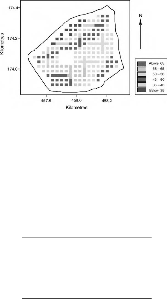
content was measured by laser diffraction grain sizing. Figure 9.1 is a scatter

map showing the sampling scheme and the percentages of sand at the sampling

points on a grey scale. There is evidently a trend across the ﬁeld. Table 9.1

summarizes the statistics. The sand content varies widely from 14% to 83%,

with a symmetric distribution that is less peaked than normal.

Case Study 205

The experimental variogram of the data computed by the usual method of

moments, equation (4.40), is shown as the plotted points in Figure 9.2(a). The

values appear to reach a sill and then increase again; the latter increase is

symptomatic of regional trend. The solid line is a model ﬁtted to lag 300 m, a

matter to which we return below.

To explore the data we ﬁtted trend surface models on the coordinates by OLS.

The linear trend surface (an inclined plane) accounts for 28% of the variance

and the quadratic accounts for more than 46%. Therefore, we assume the trend

to have a quadratic form in further analyses.

Figure 9.2(b) shows the experimental variogram of the OLS residuals from

the quadratic trend (symbols) and the ﬁtted pentaspherical function (solid line).

Table 9.2 gives the parameters of the model that we used to krige the quadratic

Figure 9.1 Scatter map of the sand content of the topsoil at Yattendon.

Table 9.1 Summary statistics for topsoil sand content (%)

at Yattendon.

Minimum 14.00

Maximum 83.00

Mean 50.84

Median 51.00

Standard deviation 14.40

Variance 207.4

Skewness 0.02

Kurtosis 0.60

Number of observations 230

206 Kriging in the Presence of Trend and Factorial Kriging