Webster R., Oliver M.A., Geostatistics for Environmental Scientists

Подождите немного. Документ загружается.

residuals. We then added back the trend to the predictions of the residuals to

give the ﬁnal estimates. These estimates are shown as a map in Figure 9.3(b),

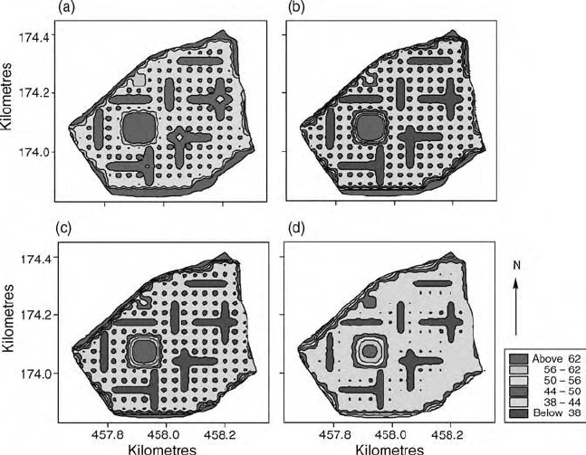
and Figure 9.4(b) is that of the associated kriging variances. The latter are for

the residuals only; they show that the estimation variances are smallest in the

region of the short transects and also at the sampling points and become large

only near the ﬁeld boundary.

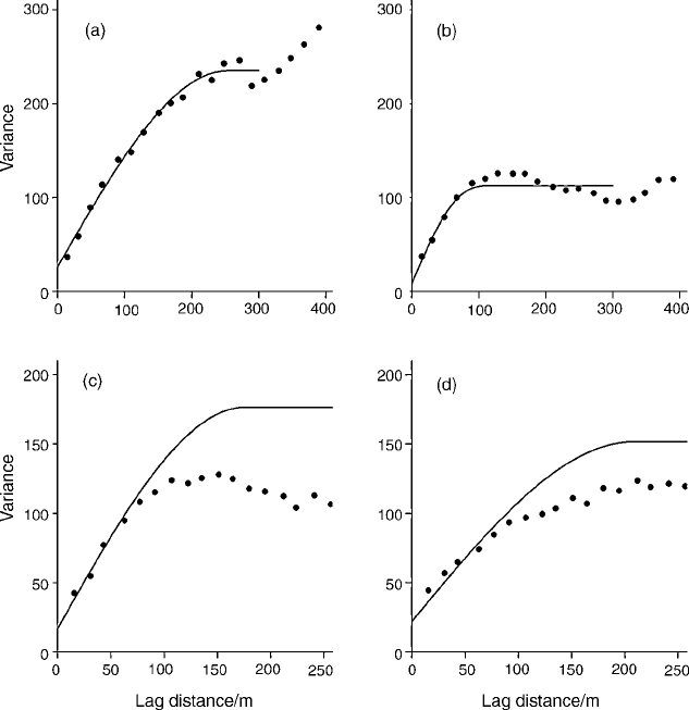
Figure 9.2 Variograms of the sand content: (a) experimental variogram computed

from the raw data by the method of moments and spherical model ﬁtted to lag 300 m;

(b) experimental variogram of the OLS residuals from a quadratic trend surface with

pentaspherical model ﬁtted; (c) variogram of the REML residuals from the quadratic

trend (solid line) with the experimental semivariances of the REML residuals plotted as

points; (d) variogram of the REML residuals after the EC

has been ﬁtted as an external

drift (solid line) with the experimental semivariances for the OLS residuals from the

external drift plotted as points.

Case Study 207

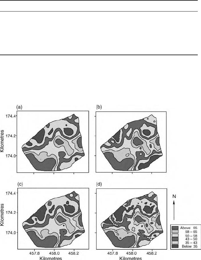
Table 9.2 Model parameters of the variograms computed on the topsoil sand content

at Yattendon. The symbols are the familar c

for the nugget variance, c for the sill of the

autocorrelated variance, and a for the range.

Variogram Model c

þ ca/m c

=ðc

þ cÞ

Raw data Spherical 27.5 208.1 235.6 254.9 0.117

OLS

residuals Pentaspherical 15.6 110.2 125.8 146.6 0.124

REML Spherical 16.6 159.8 176.4 175.8 0.104

REML

with EC

Spherical 21.7 129.9 151.6 208.7 0.167

Figure 9.3 Maps of punctually kriged estimates of sand content: (a) made by ordinary

kriging of raw data; (b) made by kriging of OLS residuals from a quadratic trend and

adding back the trend; (c) made by REML estimation, taking into account the quadratic

trend (universal kriging); (d) made by REML estimation with EC

as external drift.

208 Kriging in the Presence of Trend and Factorial Kriging

As above, dealing with trend by OLS can no longer be regarded as best

practice, and we now illustrate how do it with a REML analysis. The experi-

mental variogram of the quadratic residuals (the plotted points) and the model

estimated by REML for the residuals (the solid line) are shown in Figure 9.2(c).

We remind readers that there are no experimental semivariances for the REML

variogram. The model parameters are given in Table 9.2.

Let us now compare these models. The most marked difference is in the sill

variances, c

þ c; that for the OLS residuals is substantially smaller than that

estimated by REML. The range of the former is the shorter of the two by some 30 m.

With the parameters of the REML variogram we can now predict the sand

content by E-BLUP taking into account the quadratic trend, which is equivalent to

universal kriging, as above. Figure 9.3(c) is the resulting map, and Figure 9.4(c)

shows the associated variances.

Another variable with a strong quadratic form of trend in this ﬁeld is the soil’s

apparent electrical conductivity (EC

). This is also strongly associated with the

Figure 9.4 Maps of punctual kriging variances of sand content: (a) ordinary kriging

variances of raw data; (b) ordinary kriging variances of OLS residuals from a quadratic

trend; (c) universal kriging variances for REML estimation, taking into account the

quadratic trend; (d) variances for kriging by REML with EC

as external drift.

Case Study 209

soil’s particle size distribution. Carroll and Oliver (2005) measured the EC

an electromagnetic induction sensor, an EM38 (Geonics

Ltd—see McNeill,

1990) in the vertical position (i.e. with the coils aligned vertically), at the nodes

of a dense grid and at all the positions where sand content was recorded. The

Pearson correlation coefﬁcient computed between it and sand from collocated

data at the time of the survey was 0:8.

This strong correlation, the dense grid on which EC

was measured and the

marked trend in it make it a potentially useful external drift variable for kriging.

Our aim is to use it to improve the accuracy of the predictions of the sand

content, the primary variable.

The EC

was estimated by ordinary punctual kriging at the nodes of the

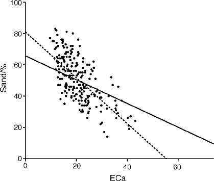
5m 5 m grid as for sand. The relation between sand content and EC

is linear,

and Figure 9.5 shows both the OLS regression (dotted) and the weighted least-

squares regression (solid) of sand on EC

. The REML variogram for sand was

computed on the random residuals from the relation. Figure 9.2(d) shows this

variogram, together with the experimental variogram of the OLS residuals, and

Table 9.2 gives the model parameters. These parameters were then used for

kriging sand with EC

on the 5 m 5 m grid as the external drift. Figure 9.3(d)

is the resulting map of estimated sand content from this analysis, and

Figure 9.4(d) shows the associated E-BLUP kriging variances.

The four variograms (Figure 9.2) appear substantially different from one

another, and their model parameters conﬁrm this impression. The variogram of

the raw data, Figure 9.2(a), has the largest sill variance. The variogram of the

OLS quadratic residuals, Figure 9.2(b), has the smallest sill variance, showing

Figure 9.5 Scatter diagram of sand content and EC

. The solid line is the weighted

least-squares regression of sand on EC

, sand ¼ 65:7  0:76  EC

, from which the

experimental semivariances in Figure 9.2(d) are computed.

210 Kriging in the Presence of Trend and Factorial Kriging

that removal of the trend has lost more of the variance than REML has done.

The REML variogram of the residuals from the quadratic trend, Figure 9.2(c),

has a larger sill variance as has the REML variogram computed on the residuals

from the relation between sand and EC

, Figure 9.2(d).

We mentioned above that there is a dearth of software in the public domain

for spatial prediction by REML. Readers, having seen Figure 9.2(a) in which

the experimental sequence of semivariances follows what looks like a

spherical form to about 300 m, and having also seen in Chapter 8 that only

data close to a target point carry signiﬁcant weight, might wonder whether

in this case they could use ordinary kriging with the raw data. Let us see

what happens if we take this approach. A spherical function, the solid line in

Figure 9.2(a), ﬁts the experimental variogram well to 300 m. Table 9.2 gives its

parameters. We used this model with the raw data to estimate values at the

nodes of the 5 m  5 m grid by ordinary punctual kriging. Figure 9.3(a) shows

the resulting map, which looks little different from those made with REML. The

map of the kriging variances, however, shows that the kriging errors are

greater.

We can summarize the four outcomes of the procedures. All four estimators

are unbiased, and because kriging is so robust the estimates themselves are

similar. They differ substantially in their variances, which are summarized in

Table 9.3. Ordinary kriging is the least precise, with a median variance of

53.1.

Universal kriging by REML reduces the variance to a median of 41.6. Kriging

with external drift has a very similar median variance, 41.3. In both, making

use of the additional information, either in the trend or in the subsidiary

correlated variable, EC

, improves the precision of the predictions. Note,

however, that the kriging variances from the KED have a smaller standard

deviation; they are less variable than those from universal kriging, and from the

other two techniques. The median kriging variance of the OLS residuals of 41.6

is remarkably similar to those of the REML predictions in this instance. Note,

however, that the OLS kriging variances underestimate the true kriging

variances of that method because the errors arising from the OLS ﬁtting of

the trend are not taken into account. The fact that they are so similar to the

REML variances is fortuitous.

Table 9.3 Summary statistics of variances for four forms of kriging.

Kriging Mean Median Std dev.

Raw data 63.2 53.1 21.0

OLS residuals 52.0 41.6 21.7

REML, universal 53.5 41.6 26.3

REML, external drift 48.2 41.3 14.6

Case Study 211

9.4 FACTORIAL KRIGING ANALYSIS

9.4.1 Nested variation

Spatial variation in the environment can occur on scales that differ by several

orders of magnitude simultaneously. This is because the physical processes

responsible for the variation operate and interact at different spatial scales. In

any region there may be several sources and scales of variability present. For

example, variation in the soil could arise from the effects of microbial activity,

worms, roots, tree-throw, relief, or geology. Variation of this kind is widespread

in the environment; for example, Serra (1968) found seven different scales of

spatial variation in the Lorraine iron ore deposit, ranging from 15 mm to several

hundred metres. The result is a nested structure in the variation that we have

already observed through the nested variogram functions in Chapter 5.

Although nested variation has been recognized for some time, there is now a

greater need than before to investigate it. This need has arisen from the

increasingly rich sets of data emerging from new technology, such as satellite

imagery, ground-penetrating radar, and sensors that measure electrical conduc-

tivity. Such data often cover large areas at an intermediate spatial resolution of

about 30 m 30 m, for example, or are very intensive, such as the 1-m pixel

resolution Hymap imagery. Because such sources of data provide full cover of the

areas of interest, nested variation is often evident (Oliver et al., 2000).

9.4.2 Theory

We can formalize nested variation in a geostatistical framework as follows. A

particular random process, ZðxÞ, may be treated as a combination of several

independent processes, one nested within another and acting at different

characteristic spatial scales. In these circumstances the variogram of ZðxÞ is

itself a nested combination of two or more, say S, individual variograms:

gðhÞ¼g

ðhÞþg

ðhÞþþg

ðhÞ; ð9: 34Þ

where the superscripts refer to the separate variograms (not powers).

If we assume that the processes are uncorrelated then we can represent

equation (9.34) by the sum of S basic variograms:

gðhÞ¼

k¼1

ðhÞ; ð9:35Þ

where g

ðhÞ is the kth basic variogram function, and b

is a coefﬁcient that

measures the relative contribution of the variance of g

ðhÞ to the sum. The

212 Kriging in the Presence of Trend and Factorial Kriging

nested variogram comprises the S variograms with different coefﬁcients b

. This

is known as the linear model of regionalization. It reﬂects the real world in

which factors such as relief, geology, the soil, vegetation, and fauna each

operate on their own characteristic spatial scale(s) and each with its particular

form and parameters, b

, for k ¼ 1; 2; ...; S.

9.4.3 Kriging analysis

The aim of kriging analysis is to estimate separately the independent compo-

nents of ZðxÞ. Matheron (1982) devised the technique of kriging analysis or

factorial kriging to do this in a single operation from the data and the

variogram. For this the random function ZðxÞ with a nested variogram is

regarded as the sum of S orthogonal random functions, each with its particular

contributory variogram, b

ðhÞ in equation (9.35). Provided ZðxÞ is second-

order stationary this sum can be represented as

ZðxÞ¼

k¼1

ðxÞþm; ð9:36Þ

in which m is the mean of the process. Each Z

ðxÞ has expectation 0, and the

squared differences are

E½fZ

ðxÞZ

ðx þhÞgfZ

ðxÞZ

ðx þ hÞg ¼

ðhÞ if k ¼ k

;

0 otherwise:

(

ð9:37Þ

It is possible that the last component, Z

ðxÞ, is intrinsic only, so that g

ðhÞ in

equation (9.35) is unbounded with gradient b

. For two components equation

(9.36) reduces to

ZðxÞ¼Z

ðxÞþZ

ðxÞþm: ð9:38Þ

Relation (9.37) expresses the mutual independence of the S random functions

ðxÞ. With this assumption, the nested model in equation (9.35) is easily

retrieved from the relation in equation (9.36).

We recall that in ordinary kriging we usually estimate Z at any place x

as a

linear combination of the n observations in the neighbourhood of x

Zðx

Þ¼

i¼1

zðx

Þ: ð9:39Þ

Factorial Kriging Analysis 213

The weights, l

; i ¼ 1; 2; ...; N, are obtained by solution of the kriging system

j¼1

gðx

; x

Þcðx

Þ¼gðx

; x

Þ for all i ¼ 1; 2; ...; n;

j¼1

¼ 1;

ð9:40Þ

in which cðx

Þ is a Lagrange multiplier introduced to ensure that the

estimation variance is minimized.

In kriging analysis we can estimate each spatial component Z

ðxÞ separately

as a linear combination of the observations zðxÞ; i ¼ 1; 2; ...; n:

ðx

Þ¼

i¼1

zðx

Þ: ð9:41Þ

The l

ðx

Þ are the weights assigned to the observations as before; but now they

must sum to 0, not to 1, to ensure that the estimate is unbiased and to accord

with equation (9.36). Subject to this condition, they are again chosen so that

the estimation variance is minimal. This leads to the kriging system

j¼1

gðx

; x

Þc

ðx

Þ¼b

ðx

; x

Þ for all i ¼ 1; 2; ...; n;

j¼1

¼ 0;

ð9:42Þ

where c

ðx

Þis the Lagrange multiplier for the kth component. This system is

solved for each spatial component, k, to ﬁnd the weights, l

, which are then

inserted into equation (9.41) for that component. In general the weights for the

different components will be different, and as a result we can extract from data

the individual components of the spatial variation that we identiﬁed from the

experimental variogram. Estimates are made for each spatial scale, i.e. each k,

by solving equations (9.42).

In many instances data contain long-range trend. This need not complicate

the analysis because the kriging is usually done in fairly small moving

neighbourhoods centred on x

, as for ordinary kriging (Chapter 8). Thus

it is necessary only that ZðxÞ is locally stationary, or quasi-stationary.

Equation (9.36) may then be rewritten as

ZðxÞ¼

k¼1

ðxÞþmðxÞ; ð9:43Þ

214 Kriging in the Presence of Trend and Factorial Kriging

where mðxÞ is a local mean which can be considered as a long-range spatial

component. Matheron (1982) showed that this relation is also veriﬁed in terms

of estimators, i.e.

ZðxÞ¼

k¼1

ðxÞþ

mðxÞ: ð9:44Þ

We have also to krige the local mean, which is again a linear combination of

the observations zðx

Þ:

mðx

Þ¼

j¼1

zðx

Þ: ð9:45Þ

The weights are obtained by solving the kriging system

j¼1

gðx

; x

Þcðx

Þ¼0 for all i ¼ 1; 2; ...; n;

j¼1

¼ 1:

ð9:46Þ

Estimation of the long-range component, i.e. the local mean mðxÞ and the

spatial component with the largest range, can be affected by the size of the

moving neighbourhood (Galli et al., 1984). In fact, to estimate a spatial

component with a given range the distance across the neighbourhood should

be at least equal to that range. It happens frequently when the sampling density

and the range are large that there are so many data within the chosen

neighbourhood that only a small proportion of them is retained. Although

modern computers can handle many data at a time, the number of data used

must be limited to avoid instabilities when inverting large variance matrices.

Further, even if all the data could be retained, only the nearest ones contribute

to the estimate because they screen the more distant data. Consequently, the

neighbourhood actually used is smaller than the neighbourhood speciﬁed,

which means that the range of the estimated spatial component is smaller

than the range apparent from the structural analysis. Galli et al. (1984)

recognized this, and where data lie on a regular grid they proposed using

only every second or every fourth point to cover a large enough area, but still

with sufﬁcient data. Such selection is somewhat arbitrary, and we recommend

an alternative proposed by Jaquet (1989) and used by Goovaerts and Webster

(1994) which involves adding to the long-range spatial component the estimate

of the local mean.

Factorial Kriging Analysis 215

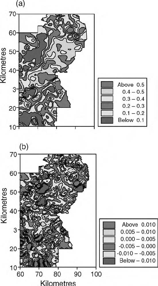
Figure 9.6 Maps of copper in the topsoil of the Borders Region of Scotland:

(a) ordinary kriged estimates; (b) estimates of short-range component; (c) estimates of

long-range component; (d) kriging variances.

216 Kriging in the Presence of Trend and Factorial Kriging