Webster R., Oliver M.A., Geostatistics for Environmental Scientists

Подождите немного. Документ загружается.

Factorial Kriging Analysis 217

9.4.4 Illustration

We illustrate factorial kriging with the available copper data in the topsoil of the

Borders Region of Scotland. These data were described in Chapter 6 to illustrate the

application of the Akaike information criterion (AIC). Table 9.4 lists the summary

statistics, which show that these data have a large skewness coefﬁcient of 2.52.

After transformation to common logarithms, log

Cu, the distribution becomes

almost normal. The experimental variogram was computed on the transformed

log

Cu values, and a double spherical function ﬁtted the experimental values best

both in terms of the mean squared residual and the AIC (Figure 5.15 and Table

5.2). This function was then used for factorial punctual kriging. We kriged at

intervals of 500 m with the maximum radius of the neighbourhood set to 20 km,

the range of the long-range spatial component. The minimum and maximum

numbers of points in the neighbourhood were set to seven and 20, respectively.

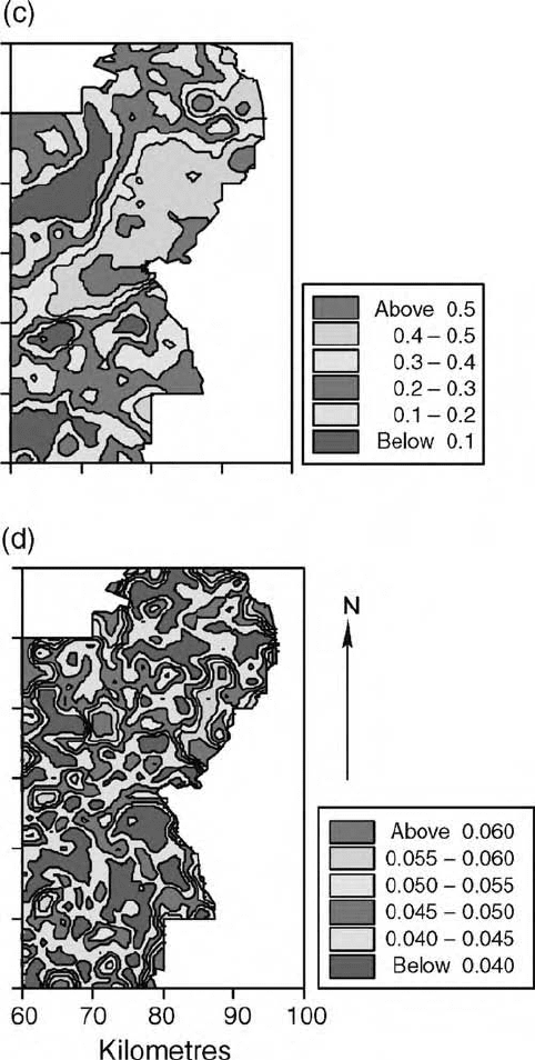
Figure 9.6(a) is a map of the punctually kriged estimates of log

Cu. There is a

band of large values that extend across the region from southwest to northeast,

with smaller concentrations of log

Cu to the north and south. The extent of

these patches of large and small concentrations represents the long-range

component of the variation of 20.5 km. These larger areas embrace many

distinct small patches of larger or smaller values which represent the short-range

component of variation of 2.7 km. Figure 9.6(b) shows the kriging variances;

these are large at the margins of the study area and in other areas where

sampling was also sparse. Figure 9.6(c) shows the short-range predictions that

have been extracted by factorial kriging. They show the more intricate local

variation that is superimposed on the broader-scale variation shown in Figure

9.6(d). It is possible to match several of the small patches of large and small

values in Figure 9.6(a) with those in Figure 9.6(c). The long-range variation is

associated with the major geological units and soil parent materials in the region.

The areas with small copper concentrations are on the sedimentary rocks of the

Old Red Sandstone, whereas on the other rocks concentrations are generally

larger. Some of the smaller patches of large Cu values are around the towns and

others are associated with outcrops of volcanic rocks.

Table 9.4 Summary statistics and variogram parameters of available copper in the

topsoil of the Borders Region of Scotland. Original measurements were in mg kg

1

soil.

Mean Median Variance Std dev. Skewness

Measurements, Cu 2.22 1.85 2.135 1.46 2.52

log

Cu 0.271 0.267 0.06502 0.255 0.06

Double spherical variogram parameters

/km a

/km

0.02767 0.02585 0.01505 2.7 20.5

218 Kriging in the Presence of Trend and Factorial Kriging

Cross-Correlation,

Coregionalization

and Cokriging

10.1 INTRODUCTION

In this chapter we develop the ideas of spatial correlation in individual variables

for use in situations in which two or more environmental variables interest us

simultaneously. We shall assume that each variable individually can be treated

as if it were random, so that all of the statistical theory and techniques of

Chapters 4–7 apply. We shall use the data from two surveys to illustrate the

development. One set comprises the exchangeable potassium (K), available

phosphorus (P) and yield of barley in the topsoil of a 6.4 ha ﬁeld in southeast

England (CEDAR Farm, Centre for Dairy Research); and the other comprises the

concentrations of potentially toxic trace metals in the Swiss Jura. Table 10.1

summarizes the data for the Farm, and Table 10.5 that of the Jura.

There are now two additional features of the variation to consider. One

comprises the relations between variables, regardless of space, as expressed in

the ordinary product-moment correlation, r , of equation (2.11). The correlation

matrix for CEDAR Farm is given in Table 10.2. Evidently K, P and yield are

related, though not strongly. In the Swiss Jura the correlations among the trace

metals in the soil are stronger (Table 10.6), and we might wish to consider

them all together in assessing the risk of pollution. The other feature concerns

the spatial aspects of this correlation: one variable may be spatially related with

another in the sense that its values at places are correlated with the values of

the other variable. For example, the potassium and phosphorus in the soil at

CEDAR Farm might be spatially correlated with the crop yield, and the

cadmium with the zinc in the Jura. In these circumstances we might be able

to take advantage of the correlation and the information contained in the

several variables to predict any one of them.

Geostatistics for Environmental Scientists/2nd Edition R. Webster and M.A. Oliver

# 2007 John Wiley & Sons, Ltd

We formalize these ideas under the general heading of coregionalization.We

start by considering two regionalized variables, Z

ðxÞ and Z

ðxÞ, which we

shall denote u and v, both obeying the intrinsic hypothesis. Thus for variable u

we have, from Chapter 4,

E½Z

ðxÞZ

ðx þ hÞ ¼ 0:

The variable will also have a variogram, speciﬁcally an autovariogram:

ðhÞ¼

E½fZ

ðxÞZ

ðx þ hÞg

: ð10:1Þ

The reason for the double uu will become apparent presently. Similarly for v, the

expected differences are 0, and its autovariogram is g

ðhÞ, consisting of the

expected squared differences in v.

The two variables will also have a cross-variogram, g

ðhÞ, deﬁned as

ðhÞ¼

E½fZ

ðxÞZ

ðx þhÞgfZ

ðxÞZ

ðx þ hÞg: ð10:2Þ

This function describes the way in which u is related spatially to v.

If both variables are second-order stationary with means m

and m

, then

both will have covariance functions:

ðhÞ¼E½fZ

ðxÞm

gfZ

ðx þ hÞm

g ð10:3Þ

Table 10.1 Summary statistics of K, P and yield of barley at CEDAR Farm based on a

sample of N ¼ 160.

K P Yield

Minimum 101.0 16.8 1.28

Maximum 243.0 89.0 4.43

Mean 155.7 49.4 3.03

Median 151.0 50.9 3.11

St. dev. 28.7 14.4 0.50

Variance 825.65 206.84 0.249

Skewness 0.91 0.24 0.72

Table 10.2 Correlation matrix for K, P and yield at

CEDAR Farm with 158 degrees of freedom.

P 0.585 1

Yield 0.329 0.395 1

K P Yield

220 Cross-Correlation, Coregionalization and Cokriging

and analogously for C

ðhÞ. They will also have a cross-covariance function:

ðhÞ¼E½fZ

ðxÞm

gfZ

ðx þ hÞm

g: ð10:4Þ

As in the univariate case, there is a spatial cross-correlation coefﬁcient,

ðhÞ, which is given by

ðhÞ¼

ðhÞ

ﬃﬃﬃﬃﬃﬃﬃﬃﬃﬃﬃﬃﬃﬃﬃﬃﬃﬃﬃﬃﬃﬃﬃﬃﬃﬃ

ð0ÞC

ð0Þ

: ð10:5Þ

Equation (10.5) is the extension of the ordinary Pearson product-moment

correlation coefﬁcient (Chapter 2) into the spatial domain for Z

ðxÞ and

ðx þhÞ. When h ¼ 0 it is the Pearson coefﬁcient. Note, however, that

ð0Þ¼0, i.e. no linear correlation in the usual sense, does not mean no

correlation at lag distances greater than zero.

Equation (10.4) contains another new feature, namely asymmetry, for in

general

E½fZ

ðxÞm

gfZ

ðx þ hÞm

g 6¼ E½fZ

ðxÞm

gfZ

ðx þ hÞm

g:

ð10:6Þ

In words, the cross-covariance between u and v in one direction is in general

different from that in the opposite direction; the function is asymmetric:

ðhÞ 6¼ C

ðhÞ or equivalently C

ðhÞ 6¼ C

ðhÞ;

since

ðhÞ¼C

ðhÞ:

Asymmetry in time is common. The temperature of the air during the day

reaches its maximum after the sun has reached its zenith and its minimum occurs

after midnight, and the air’s mean daily temperature has maxima and minima

after the solstices. There is a delay between the elevation of the sun and the

temperature of the air. Analogous asymmetry in one dimension in space is easy

to envisage. The topsoil might be related asymmetrically to the subsoil on a slope

as a result of soil creep, and irrigation by periodic ﬂooding from the same end of a

ﬁeld might redistribute salts differentially down the proﬁle. However, unless the

evidence for asymmetry is strong or there is some physical rationale for spatial

asymmetry, one might treat differences in estimates, equation (10.10) below, as

sampling effects and proceed as though the cross-correlation is symmetric.

The cross-variogram and the cross-covariance function (if it exists) are

related, and as in the univariate case the variogram can be obtained from

the covariance function by extension of equation (4.5), as follows:

ðhÞ¼C

ð0Þ

ðhÞþC

ðhÞg: ð10:7Þ

Introduction 221

However, this conversion does not retain all of the information, as we can see

by splitting the cross-covariance into an even and an odd term:

ðhÞ¼

ðþhÞþC

ðhÞg þ

ðþhÞC

ðhÞg: ð10:8Þ

The odd term, the second term on the right-hand side of equation (10.8), does

not appear in equation (10.7). Unlike the cross-covariance, therefore, the cross-

variogram is an even function, i.e. it is symmetric:

ðhÞ¼g

ðhÞ for all h:

The cross-variogram cannot express asymmetry, and it should not be used

where asymmetry is thought to be signiﬁcant.

Another way of expressing the spatial relations between the two variables is

by the codispersion coefﬁcient. For a lag h, this is

ðhÞ¼

ðhÞ

ﬃﬃﬃﬃﬃﬃﬃﬃﬃﬃﬃﬃﬃﬃﬃﬃﬃﬃﬃﬃﬃﬃﬃﬃﬃﬃ

ðhÞg

ðhÞ

: ð10:9Þ

This coefﬁcient may be thought of as the correlation between the spatial

differences of u and v. Its merit is that it is symmetric, and so its estimate

might be preferred to the cross-correlogram (10.5) for describing the cross-

correlation. For second-order stationarity, n

ðhÞ approaches r

ð0Þ as jhj

approaches inﬁnity.

10.2 ESTIMATING AND MODELLING

THE CROSS-CORRELATION

Providing there are sites where both u and v have been measured, g

ðhÞ can be

estimated in a way similar to that for autosemivariances by

ðhÞ¼

2mðhÞ

mðhÞ

i¼1

ðx

Þz

ðx

þ hÞgf z

ðx

Þz

ðx

þ hÞg: ð10:10Þ

The result is an experimental cross-variogram for u and v .

The cross-variogram can be modelled in the same way as the autovariogram,

and the same restricted set of functions is available. To describe the coregiona-

lization there is an added condition. Any linear combination of the variables is

itself a regionalized variable, and its variance must be positive or zero: it may

not be negative. This is ensured as follows.

We adopt what is called the linear model of coregionalization. In it we assume

that each variable Z

ðxÞ is a linear sum of orthogonal, i.e. independent, random

222 Cross-Correlation, Coregionalization and Cokriging

variables Y

ðxÞ, each with mean 0 and variance 1, and in which the superscript

k is simply an index, not a power:

ðxÞ¼

k¼1

j¼1

ðxÞþm

: ð10:11Þ

In this expression

E½Z

ðxÞ ¼ m

;

E½Y

ðxÞ ¼ 0 for all k and j;

and

E½fY

ðxÞY

ðx þ hÞgfY

ðxÞY

ðx þ hÞg

ðhÞ > 0fork ¼ k

and j ¼ j

;

0 otherwise:



Then the variogram for any pair of variables u and v is

ðhÞ¼

k¼1

j¼1

ðhÞ: ð10:12Þ

We can replace the products in the second summation by b

to obtain

ðhÞ¼

k¼1

ðhÞ: ð10:13Þ

These b

are the variances and covariances, i.e. nugget and sill variances, for

the independent components if they are bounded. The result might look like the

set of spherical-plus-nugget functions in Figure 10.3 below. The intercepts are

the three nugget variances, b

, and the differences between these and the

maxima are the sills of the correlated variances, b

. For unbounded variograms

the b

are the nugget variances and gradients. The coefﬁcients b

¼ b

for all

k, and for each k the matrix of coefﬁcients

must be positive deﬁnite. Since the matrix is symmetric, it is sufﬁcient that

 0 and b

 0 and that its determinant is positive or zero:

j¼jb

j

ﬃﬃﬃﬃﬃﬃﬃﬃﬃﬃﬃﬃ

This is Schwarz’s inequality.

Estimating and Modelling the Cross-Correlation 223

For V coregionalized variables the full matrix of coefﬁcients, ½b

,willbeof

order V, and its determinant and all its principal minors must be positive or zero.

Schwarz’s inequality has the following consequences for each pair of

variables:

1. Every basic structure, g

ðhÞ, represented in a cross-variogram must also

appear in the two autovariograms, i.e. b

6¼ 0 and b

6¼ 0ifb

6¼ 0. As a

corollary, if a basic structure g

ðhÞ is absent from either autovariogram,

then it may not be included in the cross-variogram.

2. The reverse is not so: b

maybezerowhenb

> 0, and structures may be

present in the autovariograms without their appearing in the cross-variogram.

In practice, ﬁtting an optimal model to the coregionalization with these

constraints seems formidable. Nevertheless, Goulard and Voltz (1992) have

provided an algorithm that converges swiftly. One chooses a suitable combina-

tion of basic variogram functions, say nugget plus spherical, and for the

autocorrelated function(s) one provides the distance parameters. These can

be approximated in advance by ﬁtting models independently to the experi-

mental variograms. Starting with reasonable values for the coefﬁcients, b

, the

computer ﬁts the model and then iterates to minimize the residual sum of

squares, checking at each step that the solution is CNSD.

As a check on the validity of a model of coregionalization one can plot the

cross experimental variogram for any pair of variables and the model for them

plus the limiting values that would hold if correlation were perfect. This last

gives what Wackernagel (2003) calls the ‘hull of perfect correlation’, and for

any pair of variables u and v it is obtained from the coefﬁcients b

and b

hull½g

ðhÞ ¼ 

k¼1

ﬃﬃﬃﬃﬃﬃﬃﬃﬃﬃﬃﬃ

ðhÞ: ð10: 14Þ

The proximity of the line of the model to the experimental points shows the

goodness of ﬁt, as before (Chapter 5). The line must also lie within the hull to be

acceptable. But perhaps most revealing is the proximity of the cross-variogram

to the hull. If the two are close then the cross-correlation is strong. If, in

contrast, the cross-variogram lies far from the bounds then the correlation is

weak. This feature may be appreciated by examining Figure 10.3, and we shall

discuss it in the ﬁrst example below.

10.2.1 Intrinsic coregionalization

In general, the ratios of the coefﬁcients to one another vary from one basic

function to another. In Figure 10.1(a), for example, we have a simple nugget-

plus-spherical variogram,

gðhÞ¼2 þ 8 sph ð1:7Þ;

224 Cross-Correlation, Coregionalization and Cokriging

shown as a solid line. If we multiply the nugget, 2, by 1.2 and the spherical

component by 2 we obtain the dashed line, which has a different shape from the

solid line. If our two multipliers are 2 and 1.2 then we obtain the dotted line,

which is of a similar shape to the ﬁrst, but with a different nugget: sill ratio. The

range is the same, but the proportions of nugget to sill are all different.

It sometimes happens, however, that all the auto- and cross-variograms are

proportional to a single variogram function, so that in terms of equation (10.13)

all the coefﬁcients b

are the same for all k for each combination of u and v,thus:

ðhÞ¼

k¼1

ðhÞ; ð10:15Þ

in which we replace the b

, k ¼ 1; 2; ...; K, by the single coefﬁcient b

. They

are simply multiples of one another with the same basic shape. As an example,

Figure 10.1(b) shows the basic spherical variogram. If we multiply the two

original components in turn by 1.2 and 2, representing b

, b

and b

, then we

obtain the two additional variograms, represented by the dashed and dotted

lines, respectively. These are the same apart from the vertical scale.

Where the variables are second-order stationary,

ðhÞ¼C

ð0ÞgðhÞ; ð10:16Þ

with gðhÞ!1asjhj!1. Spatial cross-correlation of this kind is said to be

intrinsic. The term is somewhat unfortunate in that this usage of ‘intrinsic’

differs from that in the ‘intrinsic hypothesis’.

Where spatial correlation is intrinsic the codispersion coefﬁcient n

ðhÞ

remains constant for all h, i.e.

ðhÞ¼

ﬃﬃﬃﬃﬃﬃﬃﬃﬃﬃﬃﬃ

ð0Þ

ﬃﬃﬃﬃﬃﬃﬃﬃﬃﬃﬃﬃﬃﬃﬃﬃﬃﬃﬃﬃﬃﬃﬃﬃﬃﬃ

ð0ÞC

ð0Þ

¼ n

ð0Þ:

Figure 10.1 Spherical variograms with constant range, 1.7: (a) of differing shapes and

differing nugget: sill ratios in the general case; (b) of constant nugget: sill ratios in the

intrinsic case. See text for further explanation.

Estimating and Modelling the Cross-Correlation 225

10.3 EXAMPLE: CEDAR FARM

We illustrate the procedure and some of the features of coregionalization using the

survey data of a ﬁeld on CEDAR Farm in southeast England. They derive from an

original study of precision farming by Dr Z. L. Frogbrook, who kindly provided

them and to whom we are grateful. The ﬁeld covers approximately 6.4 ha of fairly

ﬂat land on clay and is cultivated to produce cereals. Its topsoil (0–15 cm) was

sampled at 160 places on 5 m  2 m supports at 20 m intervals on a square grid.

The yield of barley was measured on the same supports in 1998. The principal

plant nutrients, exchangeable potassium (K) and available phosphorus (P), were

measured. The data are summarized in Table 10.1. Potassium and yield are

somewhat skewed, but not so seriously as to warrant transformation. The three

variables are correlated, though not strongly, as Table 10.2 shows.

By applying equation (10.10) and treating the variation as isotropic, we obtain

the experimental auto- and cross-variograms. The experimental variograms have

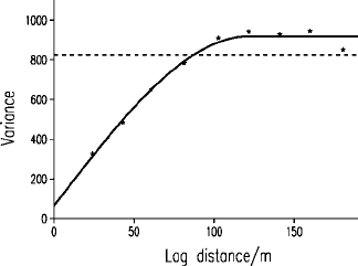
simple forms. Figure 10.2 shows an example; it is the autovariogram of K with a

spherical model ﬁtted to it by weighted least squares, as described in Chapter 5. The

model’s coefﬁcients are listed in Table 10.3. The other experimental variograms

appear in Figure 10.3 as the point symbols. Four of them, namely the autovario-

gram of yield (Figure 10.3(e)), and the three cross-variograms, Figures 10.3(b),

10.3(d) and 10.3(f), are evidently bounded, and again the spherical model ﬁtted

them well. The coefﬁcients of ﬁtting the model independently are listed in

Table 10.3. The autovariogram of P does not reach a bound within the ﬁeld.

The ﬁve bounded variograms have approximately the same range, and so we

can reasonably ﬁt the linear model of coregionalization with two basic

components, g

ð0Þ, i.e. nugget, and g

ðjhjÞ. We set the range of g

ðjhjÞ to

144 m, the average of the ﬁve bounded variogram models. The resulting

coefﬁcients b

are listed in Table 10.4, and the solid lines in Figure 10.3

are those of the linear model of coregionalization. We can see by comparing

Figure 10.2 with Figure 10.3(a) for K that the model of coregionalization ﬁts

Figure 10.2 Variogram of potassium at CEDAR Farm with experimental values plotted

as point symbols and the spherical model shown as the solid line.

226 Cross-Correlation, Coregionalization and Cokriging